Download

1 / 31
330 likes | 372 Views
Explore the climatological background state, wind forcing, thermocline structure, ENSO influences, and long-term trends in the Indian Ocean to understand its circulation and climate variability.

E N D
Indian Ocean circulation and climate variability Jay McCreary, Fritz Schott & Shang-Ping Xie Summer School on: Dynamics of the North Indian Ocean National Institute of Oceanography Dona Paula, Goa June 17 – July 29, 2010
References (SXM09) Schott, F.A., S.-P. Xie, and J.P. McCreary, 2009: Indian Ocean circulation and climate variability. Rev. Geophys., 47, RG1002, doi:10.1029/2007RG000245.
Outline Climatological background state Influence of thermocline depth Impact of ENSO in IO IO warming after ENSO Indian Ocean dipole An IO “La Nina” Longer-term variability & trends IO warming & IOD decadal variability
Climatological background state Influence of thermocline depth
Wind forcing Seasonally reversing monsoon winds Quasi-steady Southeast Trades
Thermocline structure Key regions of air-sea interaction are where the thermocline is shallow, where wind-stress variability can produce large SST anomalies. In the IO, these regions include: i) off Somalia, ii)around the tip of India, and iii) in the 5–10ºS band. Indeed, the latter region appears to very important for IO air-sea interaction. An additional region, not evident in this climatological plot, is the upwelling region off Sumatra/Java. Air-sea interaction in this region is a key process in IO Dipole (IOD) events (also known as IOZM, IODZM, and IOZDM).
SST and precipitation There is a close connection between SST and precipitation in the 5–10ºS band. During DJF, precipitation extends into the western IO where SST is warm. During JJA, it is confined to the eastern/central ocean because SST is cool in the west. SST in the 5–10ºS band is related to the thermocline depth there, the shallower and longer region during JJA cooling SST. Precipitationappears to be prevented in the west by the cool SSTs.
Impacts of ENSO in the IO IO warming after ENSO
ENSO Figure 12: Correlations between Nino3 SST for Nov(0)-Jan(1) with SST in the eastern equatorial Pacific (160W–120W, 5S–5N; black), the tropical IO (40–100E, 20S–20N; red), the Southwest IO (50–70E, 15–5S; green), and the eastern equatorial IO (90–110E, 10S–Eq.; blue). What processes cause the warming? What causes the delay? What are the impacts of these SST anomalies on the atmosphere?
ENSO January June November August The thermocline ridge is shallow throughout the year. One can expect that ENSO-related IO winds generate large SST anomaliesthere.
ENSO r(Z20,SST) There is a close connection between thermocline depthand SST in the western, tropical IO at interannual time scales. Figure 14: a) Annual-mean depth of the 20ºC isotherm (contours in m) and correlation of its interannual anomalies with local SST(color shades) (from Xie et al., 2002).
ENSO r(Z20,SST) Precipitation 15 Xie et al. (2002) The thermocline ridge provides a “window” for coupling ocean dynamics (thermocline depth) to SST and, hence, to atmospheric convection.
ENSO Xie et al. (2002) Figure 17: Correlation with eastern Pacific SST during Oct-Dec (months 10–12) as a function of x and t: Z20, SST, and rainfall averaged from 8–12ºS. Shading denotes where correlation exceeds 0.6 with Z20 in (a) and (b), and with SST in (c). The SWIO delay results from a downwelling Rossby wave generated in the southeastern IO, which deepens the pycnocline in the 5–10ºS ridge after its arrival there. As a result, SST warms there, and this warming increases rainfall.
ENSO Figure 15: Partial correlation of 1000 hPa winds (vectors) and wind curl (colors) with a) an IOD index and b) NINO3; only correlations at 99% level are shown (from Yu et al., 2005). IOD ENSO ENSO is associated with positive wind curl. It forces a downwelling Rossby wave that propagates into the SWIO to impact the 5–10ºS ridge several months later.
ENSO NIO Nino Regressions of Nino SST during NDJ(0) on SST, windand solar radiation (–precipitation) during May-Jun(1). SWIO R The SWIO convection induces a local cyclonic circulation. It also forces a cross-equatorial response with northeasterlies throughout the NIO. They weaken the SWM, causing NIO warming for the second time. There are also precipitation anomalies in the tropical WNP. As discussed next, they appear to be remotely generated by the IO warming via the radiation of an atmospheric warm Kelvin wave. Du et al. (2009, J Climate)
ENSO 850-250 mb temp, surface winds precip Xie et al. (2009, J. Climate) A warm atmospheric Kelvin wave radiates from the TIO, and because of damping generates northeasterlies and surface divergence on its northern flank, which suppresses convection over the tropical NWP.
ENSO p, (u, v) The response is represented simply by the Gill atmospheric model, which models the response of a baroclinic mode of the atmosphere to a prescribed heating. The solution has a local response and radiates damped Kelvin and Rossby waves, which are damped by Newtonian cooling (–κp).
ENSO The atmospheric modelis dry, linearizedabout the NCEP mean state for JJA, with 20 vertical levels. It is forced by a prescribed diabatic heatingthat extends throughout the troposphere, to model deep convection. SLP & sfc wind The figure shows the response to a symmetric, basin-scale heating over the TIO. As in the Gill model, a Kelvin wave radiates into the tropical WP. Northeasterlies develop on its northern flank, due to the background winds and to damping. Xie et al. (2009, J. Climate) SLP & sfc wind The figure shows the response when an additional diabatic heating is imposed in the tropical WNP that is proportional to the average wind convergence in the blue area. In this case, a pronounced anticyclonic circulation develops, consistent with the observations.
ENSO Second warming May Kelvin wave Summary JJA(1) Feb Rossby wave ENSO wind curl Ocean-atmosphere interaction in the SWIO is anchored by warming due to an oceanic Rossby wave. It is key to the persistence of the warming throughout the IO during JJA(1). The IO warming excites an atmospheric Kelvin wave, which causes low-level divergencein the tropical NWP, reducing rainfall and generating an anticyclone there.
Indian Ocean Dipole An IO “La Nina”
IOD The typical IOD develops from Sept–Nov, with dipole anomalies in SST, Z20, and precipitation and anomalous equatorial easterlies. These changes are all consistent with the occurrence of Bjerknes feedback. Figure 18: IOD pattern during Sept-Nov. a) Regression of Z20 (shading in m) and surface wind velocity (m/s) on the first principal component of Z20. b) Correlation of precip (shading) and SST (contours at 0.3, 0.6 and 0.9 and negative dashed) with the first principal component of Z20. From Saji et al. (2006a).
IOD The IOD-year curves lie outside the standard deviation of all interannual variability, supporting the idea that IOD is a climate event separate from ENSO. Why does the IOD develop in the fall (Sept–Nov)? One reason is because the normal annual cycle of SST in the EEIO is coolest (and Z20 is shallowest) at that time. Thus, the monsoon forcing creates a “window” in which IOD events can develop. Figure 21:b) Seasonal cycles of SST in the EEIO (heavy solid) with interannual variability (one standard deviation, shaded) and SST and wind during IOD years (light solid). c) Same as b), except for zonal wind on equator at 85ºE. (From Saji and Yamagata, 2003).
IOD Courtesy of Jerome Vialard
IOD The τxeq anomaly is more closely related to ΔSST(0.86) than to SOI (0.67), supporting the independence of IOD from ENSO. The correlation between the SSTE and SSTW is only 0.43 and is positive. It is negative only during IOD events. Figure 20: a)SSTW and SSTE anomalies from 1981−99. b)SSTW–SSTE and Δτxeq. c) Δτxeq and inverted SOI. Light blue shading indicates El Nino events in the Pacific (from Feng and Meyers, 2003).
IOD Submonthly OLR and the IOD are closely related, with the former being strongly reduced during IOD years (corr. coeff. 0.84). The likely cause of the linkage is that atmospheric convection is suppressed (enhanced) in the EEIO during a positive (negative) IOD phase, when SST is anomalously (cool) warm. Figure 23: Variations of the intensity of submonthly (6–30 day) OLR variability for the area 2.5–12.5S, 87.5–102.5E (solid line) and an IOD index (dashed line) during SON. Shinoda and Han ( 2005)
Summary Climatological background state Climatological thermocline depth, h, is shallow in the western Arabian Sea, southern tip of India, 5–10ºS thermocline ridge, and off Sumatra/Java. These regions areclimatically important because that is where ocean dynamics can impact SST. El Nino ENSOgenerates negative Ekman pumpingin the southeastern tropical IO. It forces a Rossby wave that deepens h, warms SST, and strengthens convection in 5–10ºS thermocline ridge during the following spring, This anomalous convection weakens the onset of the SWM in the following summer, and warms the northern IO. The second warming forces an atmospheric Kelvin wave that reduces convection in the western Pacific. Indian Ocean Dipole IOD events develop during the fall, when h off Sumatra/Java is at its climatological minimum. Bjerknes feedback appears to be active during large IOD events, so that IOD is dynamically similar to a Pacific “La Nina.” During IOD events, submonthly atmospheric variability decreases significantly.
Longer-term variability and trends IO warming and IOD decadal variability
Indian Ocean warming trend From 40–50º, there was a strong, near-surface, warming trend in the western subtropical IO, an increase of 1–2ºC over 40 years extending to 800 m(panel c). In addition, from 35ºS to 5ºN there were regions of cooling below 100 m. A similar subsurface cooling pattern occurs in an average of several IPCC models (panel e). The cooling regions must involve shifts the ocean’s response to changing dynamical forcing (e.g., winds and across-boundary transports) (panel d). Alory et al. (2007) Figure 24: c) Zonally averaged temperature trends 1960–99 (shading) from new IO temperature archive (IOTA). d) as b) but calculated after shifting mean temperature structure southward by 0.5º. e) trends from mean of 10 IPCC models.
Indian Ocean warming trend The NIO heat storage has remained roughly constant in the upper 700 m over the past 50 years but has increased in the SIO. Barnett et al. (2005) suggested that stronger concentrations of aerosols over the northern IO weakened the climate-change signal there. Figure 24: Time series of yearly heat content in the upper 700 m for a) the SIO and b) the NIO, with vertical bars for 1 std. dev. of the annual means, red line the respective trends and numbers explained variance by trend line (from Levitus et al., 2005).
IOD decadal variability IOD events tend to cluster in decades when the EEIO is preconditioned with a shallow thermocline, thereby favoring Bjerknes feedback in the IO. The preconditioning was driven by Pacific decadal variability, both by an atmospheric bridge and by changes in the ITF. Figure 27: Thermocline-depth anomalies hin the EEIO (10ºS–0; 90–110ºE) in a) ocean GCM driven by NCEP winds. b) in the SODA reanalysis; vertical lines mark IOZM occurrences. Annamalai et al. (2005b)
Summary IO warming The 50-year warming trend in the IO is due to surface heating. Regions of subsurface cooling must result from ocean dynamics (e.g., changes in wind or across-boundary transports). The north IO has not shown significant warming for reasons that are not yet clearly understood. IO decadal variability IOD events tend to occur in decades when the EEIO thermocline is anomalously shallow, thereby favoring Bjerknes feedback.