Download
1 / 62
650 likes | 896 Views
Functional Magnetic Resonance Imaging. Jan Petr (Jan Kybic , Emily Falk, Tor Wager, Scott Huettel ). Department of Position Emission Tomography Institute of Radiopharmaceutical Cancer Research Helmholtz-Zentrum Dresden-Rossendorf. What is functional MRI (fMRI).

E N D
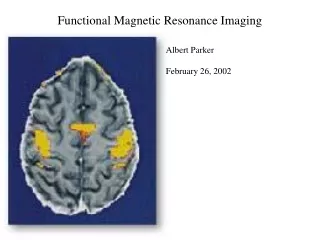
Functional Magnetic Resonance Imaging Jan Petr (Jan Kybic, Emily Falk, Tor Wager, Scott Huettel) Department of Position Emission Tomography Institute of Radiopharmaceutical Cancer Research Helmholtz-Zentrum Dresden-Rossendorf
What is functional MRI (fMRI) • Using a standard MRI scanner to image brain activity through changes in blood oxygenation or perfusion. • Non-invasive, no ionizing radiation. • Good combination of spatial and temporal resolution. • 3x3x3 mm3 voxels. • Repetition time in order of seconds.
Contents • Brain anatomy • Motivation to study brain • Applications • Methods of function localization • Hypercapnia BOLD • Arterial spin labeling
Brain anatomy • Brain – center of nervous system. • Composed of neurons and neuroglia. • Neurons communicate through axons using electrochemical processes (from mm to m).
Brain anatomy • Gray matter • Consists mostly of neurons. • Cerebral cortex of cerebrum and cerebellum. • Processing and cognition function. • White matter • Consists mostly of axons. • Connects gray matter regions.
Brain anatomy • Blood supplies brain with oxygen, glucose and other nutrients.
Brain anatomy • Brain regions Purves et al., Life: The Science of Biology, 4th Edition
Motivation • Investigating brain physiology • Understanding the cognition processes • Studying brain development • Improving clinical procedures
Applications • Brain Tumors • Direct: Mapping of functional properties of adjacent tissue • Indirect: Understanding of likely consequences of a treatment • Drug Abuse/Addiction • Understanding of brain effects of long-term use • Development of treatment strategies for abusers • Drug Studies • What are the effects of a given medication on the brain? • How does a drug affect cognition? … our measures of cognition? • Neuropsychological disorders • Understanding brain function may allow distinction among subtypes. • Identifying markers for a disorder may help in treatment • Aging and brain development • Which are normal changes are which are pathological
Applications • Surgery planning Patient with glioblastoma Volunteer
Applications • Standard brain mapping tasks From Hirsch, J. et al; Neurosurgery 47: 711-22, 2000.
Methods for localizing brain function • Invasive • Consequences of accidents or surgeries. • Direct cortical stimulation. • Non-invasive • MEG, EEG • fMRI • PET • NIRS
MEG/EEG • Measuring postsynaptic potentials of neurons. • Order of 100.000 neurons are needed to generate detectable change. • EEG – Electrical activity on the scalp. • MEG – magnetic fields. MEG at NIH EEG
Positron emission tomography (PET) • Injection of a tracer (e.g. 18F-FDG) • + Biologically active molecule (e.g. glucose) • + radioisotope (e.g. fluorine-18 isotope) • Tracer accumulation in cells. • β+ decay a positron is emitted • Positron + electron annihilation • Pair of γ photons emitted in opposite direction (energy 511keV) • Detection coincidences using scintillator and photomultiplier. • Reconstruction of 3D decay distribution using EM algorithm or filtered back-projection.
Functional studies with PET • Quantitative study of metabolic rates. • Previous PET images – static PET • cca 1h waiting after injections • Decay corrected measurement of activity, normalized to SUV • 15O-H2O (half-life 122 seconds) • Oxygen metabolism. • 18F-FDG • Glucose metabolism. • Advantages • Absolute metabolic rates. • Disadvantages • Invasive • Limited repeatability • Very low temporal resolution Duke UNC
NIRS • Near infrared spectroscopy (Jöbsis, 1977). • Biological tissue is relatively transparent to light with 700-900nm. • Can penetrate skull and brain several cm deep. • Is scattered and partly absorbed on the way. • Oxygenated and deoxygenated hemoglobin, cytochrome-C-oxidase Images: Stefanie Zechner, CeyhunBurakAkgül.
History of fMRI • Blood Oxygenation Level Dependent. • Indirect measurement correlated with neuronal activity. Angelo Mosso 1881 – Observed changes of cerebral blood flow during mental activity Linus Pauling 1936 – Discovered magnetic properties of haemoglobin Peter Mansfield 1973 – Participated in discovery of Magnetic resonance imaging 1977 – Proposed Echo Planar Imaging (EPI) Siege Ogawa 1991 – Discovered BOLD signal
First BOLD measurements • Ogawa et al., 1990 • Mice and rats at 7T MRI • Contrast on gradient-echo images influenced by proportion of oxygen in breathing gas. • Increasing oxygen content reduced contrast. • Ogawa et al., 1992 • Humans at 4T MRI • Visual stimulation • Changes of contrast in visual cortex
BOLD signal and T2* • T2* relaxation – decay of signal after excitation. • Two components of T2: • Intermolecular interactions dephasing T2 signal decay. • Macroscopic stating magnetic field inhomogeneity T2’ decay. • Relaxation rate
BOLD signal and T2* • Deoxyhaemoglobin is paramagnetic, oxyhaemoglobin is diamagnetic. • Irons binds the oxygen. • Higher dxHgb concentration increased magnetic susceptibility increased magnetic field inhomogeneities decrease T2* decreases signal. Thulborn et al., 1982 Decreasing signal Decreasing relaxation time Increasing blood oxygentation
BOLD during neuronal activity Physiological effects Brain function Metabolic rates Physical effects MR properties Neuronal activity Glucose and oxygen metabolism Cerebral blood volume (CBV) Magnetic field uniformity Decay Time (T2*) Cerebral blood flow (CBF) Blood oxygenation T2* weighted image intensity - +
BOLD during neuronal activity • Increased CBF in the activated region. • Increased production of dxHgb(removed by increased CBF). • Per volume concentration of dxHgb decreases. • Mainly in veins. Image:psychcentral.com
Hemodynamic response • Change in BOLD signal is not immediately after activation. • Differs between subjects and within subject. • Initial dip – increase in oxygen consumption before CBF increase. • Undershoot – CBF decrease faster than CBV. Peak Rise Undershoot Baseline Peak Sustained response Rise Baseline Undershoot Initial dip
fMRI study design • BOLD signal – combination of many things – CBV, CBF, O2 metabolism rate (CMRO2) etc. • Cannot be simply quantified. • Observe change of BOLD signal as a reaction on a task or event. Stimulus HRF Expected response Images:Tor Wager Hirsch J. et al. Neurosurgery 47. 711-22.2000
fMRI experimental design • Goals: To detect what is active.
Block design • Different cognitive processes segregated into distinct time periods • Task A/ Task B / Task A / Task B • Good to differentiate between conditions. • Do not see common activity. • Task A/ rest / Task A / rest … • Disadvantages: • Sensitive to choice of baseline, signal drift, head motion.
Event-related design • Associate brain processes with discrete events that may occur at any point in the scanning session. • Responses to brief event are almost always weaker than responses to blocks of events.
Event-related design Long constant response shows memory maintenance Items to remember • Consider that HRF has long delay (2-3 s) and duration (8-16 s). • Event-related fMRI with fixed timing (typically 10-20s) or with randomized timing (jittered). • Distinguishing between subtasks. • Overlapping responses superimpose. Memory probe Response to each stimuli show item encoding/recognition Combined response by superposition of individual responses Responses to individual events Events
Event-related design • Advantages • Avoids habituation issues. • Flexible. • Self-paced tasks. • Can analyze correct/incorrect responses separately. • Disadvantages • Reduced sensitivity relative to blocked design. • Sensitive to accuracy of shape of HRF. • Short intervals may cause non-linear behavior.
Mixed design • Combination of block and event-related designs. • Best combination for detection and estimation. Donaldson et al., 2001
Preprocessing • Correcting for non-task related variability in data. • Correct for head motion • 6 parameters rigid transformation – 3 translations, 3 rotations. • Spatial normalization • To MNI template (Montreal Neurological Institute) – approximated to the Talairach space (single segmented subject) • Larger population – detect more than in single subjects. MNI template Normalized data
Preprocessing • Temporal filtering with high pass filter – to avoid baseline changes. • Spatial smoothing • Convolution with a Gaussian kernel. • Improves SNR/reduces spatial resolution.
fMRI evaluation • Block design expected response. • Correlate model at each voxel separately. • Measure residual noise variance • t-statistic = model fit / noise amplitude • Threshold t-stats and display map
fMRI signal and noise • Types of noise: • Thermal noise • Head motion • Physiological changes • Artifacts • Signal to noise ratio (SNR) Task-related variability SNR = Non-task-related variability
fMRI Generalized linear model (GLM) • Block design experiment with a language task. • 3 tasks: • Word generation: Noun presented on screen – verb generated. • Word shadowing: Noun presented on screen – thinking on it. • Rest. Generation Shadowing Rest Images: JesperAndersson Time
Generalized linear model • Generalized linear regression model. Noise Measured data Amplitude (to solve for) Design model
GLM – regressors – X Voxel with this response is responsible for word generation Word shadowing voxel Resting voxel
Generalized linear model • Fitting the model to the measured data – estimating betas. 2 3 4 0 1 0 1 0 1 2 β1∙ + β2∙ + β3∙ ≈
Generalized linear model • Bad fit. 2 3 4 0 1 0 1 0 1 2 β1∙ + β2∙ + β3∙ ≈ 0 0 3
Generalized linear model • Active in word generation. 2 3 4 0 1 0 1 0 1 2 β1∙ + β2∙ ≈ + β3∙ 0.83 0.16 2.98
Generalized linear model • Active in word generation and shadowing. 1 2 3 0 1 0 1 0 1 2 β1∙ + β2∙ + β3∙ ≈ 0.68 0.82 2.17
Generalized linear model • Voxel not active. 1 2 3 0 1 0 1 0 1 2 β1∙ + β2∙ + β3∙ ≈ 0.03 0.06 2.04
beta_0001.img ... Time-series beta_0002.img ResMS.img ... beta_0003.img Generalized linear model – fitting error
Generalized linear model • Why is error important? • Which series should we trust? β1=1 σ=0.2 n=60 β1=1 σ=0.5 n=60 β1=1 σ=0.2 n=15 β1=0.3 σ=0.2 n=60
GLM – statistics • Is there some effect? c =[1 0 0]. Is • Alternative hypothesis – what we expect to find in the data. • Null hypothesis – what you not expect to find if the alternative hypothesis is consistent with reality. • We want to reject the null hypothesis. • Calculate the t-contrast:
Statistics • t-contrast – follows Student’s t-distribution with n-1 degrees of freedom. • P-value - How likely is to draw null hypothesis is true. • For 100 observations, we can reject the null hypothesis at 95% confidence for t>2.009
GLM – t-contrast • Voxels activated in word generation. • c = [1 0 0]
GLM – t-contrast • Voxels activated in more in word generation than in shadowing. • c = [1 -1 0]