Download

1 / 39
390 likes | 416 Views
Exploring population parameters with t-distributions; calculating standard deviation; using t-values for inference in real data studies

E N D
Inference for Distributions- for the Mean of a Population Chapter 7.1
Sweetening colas Cola manufacturers want to test how much the sweetness of a new cola drink is affected by storage. The sweetness loss due to storage was evaluated by 10 professional tasters (by comparing the sweetness before and after storage): Taster Sweetness loss • 1 2.0 • 2 0.4 • 3 0.7 • 4 2.0 • 5 −0.4 • 6 2.2 • 7 −1.3 • 8 1.2 • 9 1.1 • 10 2.3 Obviously, we want to test if storage results in a loss of sweetness, thus: H0: m = 0 versus Ha: m > 0 • This looks familiar. However, here we do not know the population parameter s. • The population of all cola drinkers is too large. • Since this is a new cola recipe, we have no population data. This situation is very common with real data.
When the sample size is large, the sample is likely to contain elements representative of the whole population. Then s is a good estimate of s. But when the sample size is small, the sample contains only a few individuals. Then s is a mediocre estimate of s. When s is unknown The sample standard deviation s provides an estimate of the population standard deviation s. Populationdistribution Large sample Small sample
A study examined the effect of a new medication on the seated systolic blood pressure. The results, presented as mean ± SEM for 25 patients, are 113.5 ± 8.9. What is the standard deviation s of the sample data? Standard deviation s – standard error s/√n For a sample of size n,the sample standard deviation s is: n − 1 is the “degrees of freedom.” The value s/√n is called the standard error of the mean SEM. Scientists often present sample results as mean ± SEM. SEM = s/√n <=> s = SEM*√n s = 8.9*√25 = 44.5
The t distributions Suppose that an SRS of size n is drawn from an N(µ, σ) population. • When s is known, the sampling distribution is N(m, s/√n). • When s is estimated from the sample standard deviation s, the sampling distribution follows at distribution t(m, s/√n) with degrees of freedom n − 1. is the one-sample t statistic.
When n is very large, s is a very good estimate of s, and the corresponding t distributions are very close to the normal distribution. The t distributions become wider for smaller sample sizes, reflecting the lack of precision in estimating s from s.
Standardizing the data before using Table D As with the normal distribution, the first step is to standardize the data. Then we can use Table D to obtain the area under the curve. Here, m is the mean (center) of the sampling distribution, and the standard error of the mean s/√n is its standard deviation (width).You obtain s, the standard deviation of the sample, with your calculator. t(m,s/√n) df = n − 1 t(0,1)df = n − 1 1 s/√n m t 0
When σ is unknown, we use a t distribution with “n−1” degrees of freedom (df). Table D shows the z-values and t-values corresponding to landmark P-values/ confidence levels. When σ is known, we use the normal distribution and the standardized z-value. Table D
Table D gives the area to the RIGHT of a dozen t or z-values. It can be used for t distributions of a given df and for the Normal distribution. (…) Table A vs. Table D Table A gives the area to the LEFT of hundreds of z-values. It should only be used for Normal distributions. (…) Table D Table D also gives the middle area under a t or normal distribution comprised between the negative and positive value of t or z.
The one-sample t-confidence interval The level Cconfidence interval is an interval with probability C of containing the true population parameter. We have a data set from a population with both m and s unknown. We use to estimate m and s to estimate s, using a t distribution (df n−1). Practical use of t : t* • C is the area between −t* and t*. • We find t* in the line of Table D for df = n−1 and confidence level C. • The margin of error m is: C m m t*
Red wine, in moderation Drinking red wine in moderation may protect against heart attacks. The polyphenols it contains act on blood cholesterol, likely helping to prevent heart attacks. To see if moderate red wine consumption increases the average blood level of polyphenols, a group of nine randomly selected healthy men were assigned to drink half a bottle of red wine daily for two weeks. Their blood polyphenol levels were assessed before and after the study, and the percent change is presented here: Firstly: Are the data approximately normal? There is a low value, but overall the data can be considered reasonably normal.
What is the 95% confidence interval for the average percent change? (…) Sample average = 5.5; s = 2.517; df = n − 1 = 8 The sampling distribution is a t distribution with n − 1 degrees of freedom. For df = 8 and C = 95%, t* = 2.306. The margin of error m is: m = t*s/√n = 2.306*2.517/√9 ≈ 1.93. With 95% confidence, the population average percent increase in polyphenol blood levels of healthy men drinking half a bottle of red wine daily is between 3.6% and 7.6%. Important: The confidence interval shows how large the increase is, but not if it can have an impact on men’s health.
The one-sample t-test As in the previous chapter, a test of hypotheses requires a few steps: • Stating the null and alternative hypotheses (H0 versus Ha) • Deciding on a one-sided or two-sided test • Choosing a significance level a • Calculating t and its degrees of freedom • Finding the area under the curve with Table D • Stating the P-value and interpreting the result
One-sided (one-tailed) Two-sided (two-tailed) The P-value is the probability, if H0 is true, of randomly drawing a sample like the one obtained or more extreme, in the direction of Ha. The P-value is calculated as the corresponding area under the curve, one-tailed or two-tailed depending on Ha:
For df = 9 we only look into the corresponding row. The calculated value of t is 2.7. We find the 2 closest t values. 2.398 < t = 2.7 < 2.821 thus 0.02 > upper tail p > 0.01 Table D For a one-sided Ha, this is the P-value (between 0.01 and 0.02); for a two-sided Ha, the P-value is doubled (between 0.02 and 0.04).
Sweetening colas (continued) Is there evidence that storage results in sweetness loss for the new cola recipe at the 0.05 level of significance (a = 5%)? H0: = 0 versus Ha: > 0 (one-sided test) The critical value ta = 1.833.t > ta thus the result is significant. 2.398 < t = 2.70 < 2.821 thus 0.02 > p > 0.01.p < athus the result is significant. The t-test has a significant p-value. We reject H0. There is a significant loss of sweetness, on average, following storage. Taster Sweetness loss 1 2.0 2 0.4 3 0.7 4 2.0 5 -0.4 6 2.2 7 -1.3 8 1.2 9 1.1 10 2.3 ___________________________ Average 1.02 Standard deviation 1.196 Degrees of freedom n − 1 = 9
Sweetening colas (continued) Minitab
Matched pairs t procedures Sometimes we want to compare treatments or conditions at the individual level. These situations produce two samples that are not independent — they are related to each other. The members of one sample are identical to, or matched (paired) with, the members of the other sample. • Example: Pre-test and post-test studies look at data collected on the same sample elements before and after some experiment is performed. • Example: Twin studies often try to sort out the influence of genetic factors by comparing a variable between sets of twins. • Example: Using people matched for age, sex, and education in social studies allows canceling out the effect of these potential lurking variables.
In these cases, we use the paired data to test the difference in the two population means. The variable studied becomes Xdifference = (X1−X2), andH0: µdifference= 0 ; Ha: µdifference>0 (or <0, or ≠0) Conceptually, this is not different from tests on one population.
Sweetening colas (revisited) The sweetness loss due to storage was evaluated by 10 professional tasters (comparing the sweetness before and after storage): Taster Sweetness loss • 1 2.0 • 2 0.4 • 3 0.7 • 4 2.0 • 5 −0.4 • 6 2.2 • 7 −1.3 • 8 1.2 • 9 1.1 • 10 2.3 We want to test if storage results in a loss of sweetness, thus: H0: m = 0 versus Ha: m > 0 Although the text didn’t mention it explicitly, this is a pre-/post-test design and the variable is the difference in cola sweetness before minus after storage. A matched pairs test of significance is indeed just like a one-sample test.
11 “difference” data points. Does lack of caffeine increase depression? Individuals diagnosed as caffeine-dependent are deprived of caffeine-rich foods and assigned to receive daily pills. Sometimes, the pills contain caffeine and other times they contain a placebo. Depression was assessed. • There are 2 data points for each subject, but we’ll only look at the difference. • The sample distribution appears appropriate for a t-test.
H0: mdifference = 0 ; H0: mdifference > 0 Does lack of caffeine increase depression? For each individual in the sample, we have calculated a difference in depression score (placebo minus caffeine). There were 11 “difference” points, thus df = n − 1 = 10. We calculate that = 7.36; s = 6.92 For df = 10, 3.169 < t = 3.53 < 3.581 0.005 > p > 0.0025 Caffeine deprivation causes a significant increase in depression.
Robustness The t procedures are exactly correct when the population is distributed exactly normally. However, most real data are not exactly normal. The t procedures are robust to small deviations from normality – the results will not be affected too much. Factors that strongly matter: • Random sampling. The sample must be an SRS from the population. • Outliers and skewness. They strongly influence the mean and therefore the t procedures. However, their impact diminishes as the sample size gets larger because of the Central Limit Theorem. Specifically: • When n < 15, the data must be close to normal and without outliers. • When 15 > n > 40, mild skewness is acceptable but not outliers. • When n > 40, the t-statistic will be valid even with strong skewness.
(B) Population Sample 2 Sample 1 Comparing two samples (A) Population 1 Population 2 Sample 2 Sample 1 Which is it? We often compare two treatments used on independent samples. Is the difference between both treatments due only to variations from the random sampling (B), or does it reflect a true difference in population means (A)? Independent samples: Subjects in one samples are completely unrelated to subjects in the other sample.
Two-sample z statistic We have two independent SRSs (simple random samples) possibly coming from two distinct populations with (m1,s1) and (m2,s2). We use 1 and 2 to estimate the unknown m1 and m2. When both populations are normal, the sampling distribution of ( 1−2) is also normal, with standard deviation : Then the two-sample z statistic has the standard normal N(0, 1) sampling distribution.
Two independent samples t distribution We have two independent SRSs (simple random samples) possibly coming from two distinct populations with (m1,s1) and (m2,s2) unknown. We use ( 1,s1) and ( 2,s2) to estimate (m1,s1) and (m2,s2), respectively. To compare the means, both populations should be normally distributed. However, in practice, it is enough that the two distributions have similar shapes and that the sample data contain no strong outliers.
The two-sample t statistic follows approximately the t distribution with a standard error SE (spread) reflecting variation from both samples: Conservatively, the degrees of freedom is equal to the smallest of (n1 − 1, n2 − 1). df m1-m2
Two-sample t significance test The null hypothesis is that both population means m1 and m2 are equal, thus their difference is equal to zero. H0: m1 = m2 <=> m1−m2 = 0 with either a one-sided or a two-sided alternative hypothesis. We find how many standard errors (SE) away from (m1−m2) is ( 1−2) by standardizing with t: Because in a two-sample test H0poses (m1−m2) = 0, we simply use With df = smallest(n1 − 1, n2 − 1)
Does smoking damage the lungs of children exposed to parental smoking? Forced vital capacity (FVC) is the volume (in milliliters) of air that an individual can exhale in 6 seconds. FVC was obtained for a sample of children not exposed to parental smoking and a group of children exposed to parental smoking. We want to know whether parental smoking decreases children’s lung capacity as measured by the FVC test. Is the mean FVC lower in the population of children exposed to parental smoking?
H0: msmoke = mno <=> (msmoke−mno) = 0 Ha: msmoke < mno <=> (msmoke−mno) < 0 (one sided) The difference in sample averages follows approximately the t distribution: We calculate the t statistic: In table D, for df 29 we find:|t| > 3.659 => p < 0.0005 (one sided) It’s a very significant difference, we reject H0. Lung capacity is significantly impaired in children of smoking parents.
C mm −t* t* Two-sample t confidence interval Because we have two independent samples we use the difference between both sample averages ( 1 −2) to estimate (m1−m2). Practical use of t: t* • C is the area between −t* and t*. • We find t* in the line of Table D for df = smallest (n1−1; n2−1) and the column for confidence level C. • The margin of error m is:
Common mistake !!! A common mistake is to calculate a one-sample confidence interval for m1 and then check whether m2 falls within that confidence interval, or vice-versa. This is WRONG because the variability in the sampling distribution for two independent samples is more complex and must take into account variability coming from both samples. Hence the more complex formula for the standard error.
Can directed reading activities in the classroom help improve reading ability? A class of 21 third-graders participates in these activities for 8 weeks while a control classroom of 23 third-graders follows the same curriculum without the activities. After 8 weeks, all children take a reading test (scores in table). 95% confidence interval for (µ1 − µ2), with df = 20 conservatively t* = 2.086: With 95% confidence, (µ1 − µ2), falls within 9.96 ± 8.99 or 1.0 to 18.9.
Robustness The two-sample t procedures are more robust than the one-sample t procedures. They are the most robust when both sample sizes are equal and both sample distributions are similar. But even when we deviate from this, two-sample tests tend to remain quite robust. When planning a two-sample study, choose equal sample sizes if you can. As a guideline, a combined sample size (n1 + n2) of 40 or more will allow you to work with even the most skewed distributions.
Details of the two sample t procedures The true value of the degrees of freedom for a two-sample t-distribution is quite lengthy to calculate. That’s why we use an approximate value, df = smallest(n1 − 1, n2 − 1), which errs on the conservative side (often smaller than the exact). Computer software, though, gives the exact degrees of freedom—or the rounded value—for your sample data.
Pooled two-sample procedures There are two versions of the two-sample t-test: one assuming equal variance (“pooled 2-sample test”)and one not assuming equal variance (“unequal” variance, as we have studied)for the two populations. They have slightly different formulas and degrees of freedom. The pooled (equal variance) two-sample t-test was often used before computers because it has exactly the t distribution for degrees of freedom n1 + n2− 2. However, the assumption of equal variance is hard to check, and thus the unequal variance test is safer. Two normally distributed populations with unequal variances
When both population have the same standard deviation, the pooled estimator of σ2 is: The sampling distribution for (x1 − x2) has exactly the t distribution with (n1 + n2 − 2) degrees of freedom. A level C confidence interval for µ1 − µ2 is (with area C between −t* and t*) To test the hypothesis H0: µ1 = µ2against a one-sided or a two-sided alternative, compute the pooled two-sample t statistic for the t(n1 + n2 − 2) distribution.
Comparing vitamin content of bread immediately after baking vs. 3 days later (the same loaves are used on day one and 3 days later). Comparing vitamin content of bread immediately after baking vs. 3 days later (tests made on independent loaves). Average fuel efficiency for 2005 vehicles is 21 miles per gallon. Is average fuel efficiency higher in the new generation “green vehicles”? Is blood pressure altered by use of an oral contraceptive? Comparing a group of women not using an oral contraceptive with a group taking it. Review insurance records for dollar amount paid after fire damage in houses equipped with a fire extinguisher vs. houses without one. Was there a difference in the average dollar amount paid? Which type of test? One sample, paired samples, two samples?