Download
1 / 63
630 likes | 774 Views
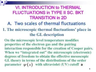
VI. INTRODUCTION to THERMAL FLUCTUATIONS in TYPE II SC. BKT TRANSITION in 2D. A. Two scales of thermal fluctuations. 1. The microscopic thermal fluctuations’ place in the GL description.

E N D
VI. INTRODUCTION to THERMAL FLUCTUATIONS in TYPE II SC. BKT TRANSITION in 2D A. Two scales of thermal fluctuations 1. The microscopic thermal fluctuations’ place in the GL description On the microscopic level temperature modifies properties of the electron gas and the pairing interaction responsible for the creation of Cooper pairs. When we “integrated out” the microscopic (electronic) degrees of freedom to obtain the effective mesoscopic GL theory in terms of the distributions of the order parameter with ultraviolet (UV) cutoff a
One loosely describes the effective mesoscopic order parameter as a classical field of Cooper pairs with center of mass at x. More mathematically, the remaining mesoscopic part of the statistical sum obeys the “scale matching”:
Quantum effects on the mesoscopic level are usually small (only when temperature is very close to T=0 they might be of importance) and will be neglected. In this case the mesoscopic classical field is independent of time. Dynamical generalization of the GL approach will be introduced later.
The coefficients of the GL energy are dependent on temperature expressing these “microscopic” thermal fluctuations. The dependence can, in principle, be derived from a microscopic theory (example: Gor’kov’s derivation from the BCS theory of “conventional superconductors). The coefficients also depend on UV cutoff L or a, but we will see that this dependence can be “renormalized away”. In practice the “constants” are also weakly (typically logarithmically) temperature dependent
leading for example to “curving down” of the Hc2(T) line: Normal Mixed state Meissner
2. Two kinds of mesoscopic thermal fluctuations: “perturbative” and “topological” The mesoscopic fluctuations qualitatively are of two sorts: “perturbative” small ones and “topologically nontrivial” or vortex ones. Since under magnetic field the order parameter takes a form of vortices, the mesoscopic fluctuations can be qualitatively viewed as distortions of a system of vortices or “thermal motion”: vibrations, rotations, waves.
Major thermal fluctuations effects include broadening of the resistivity drop (paraconductivity) and diamagnetism in the normal phase and melting of the vortex solid into a homogeneous vortex liquid state Resistance Broadening of the resistivity Nonfluctuating SC Normal Metal FluctuatingSC TC T Magnetization or conductivity are greatly enhanced in the “normal” region due to thermally generated “virtual” Cooper pairs.
Influence of the fluctuations on the vortex matter phase diagram Due to the thermally induced vibrations lattice can melt into “vortex liquid” and the vortex matter phase diagram becomes more complicated.
H E2 breaking Just crossover FLL Normal U(1) breaking Vortex liquid Meissner T Symmetries broken at the two transitons Since symmetry of the normal and liquid phases are same, the normal – liquid line becomes just a crossover. Two different symmetries are at play: the geometrical E(2) (including translations and rotations) and the electric charge U(1).
B. Nontopological excitations. The Ginzburg criterion. 1. Gaussian fluctuations around the Meissner state We ignore the thermal fluctuations of the magnetic field which turn out to be very small even for high Tc SC in magnetic field. The effect of thermal fluctuations on the mesoscopic scale is determined by
Ginzburg number It is convenient to use units of coherence length (which might be different in different directions), Y in units of Y0 and energy scale in units of critical temperature In the new units the Boltzmann factor becomes:
with the anisotropy parameter Here an important dimensionless parameter characterizing strength of thermal fluctuations is Where the temperature independent Ginzburg number characterizing he material was introduced:
Perturbation theory To calculate the thermal effects via a somewhat bulky functional integral, the simplest method is the saddle point evaluation assuming that w is small. One minimized the free energy around the “classical” or nonfluctuating solution (which we found in the preceding parts also for the SC phase) and then expands in “small” fluctuations”
Now we consider the normal phase t>1 in which the saddle point value of the order parameter is trivial: The thermal average of the order parameter is still zero due to the U(1) symmetry: However the superfluid density due to fluctuations. First we calculate the fluctuation correction to free energy and thereby to specific heat which is impacted the most.
The fluctuation contribution to free energy From now on fl is dropped. The expansion of the partition function results in gaussian integrals:
which is presented graphically as “diagrams”: It is more convenient to perform the calculation in momentum space
since the basic gaussian integral in momentum space becomes a product The leading order Therefore the fluctuations contribution to the free energy density is:
The fact that free energy depends on the UV cutoff a means that it is not a directly measurable mesoscopic quantity: energy differences or derivatives are. Entropy and specific heat The mesoscopic Cooper pairs contribution to the entropy density is less dependent on the division of degrees of freedom into micro and meso: just a constant
The second derivative, the fluctuation contribution to specific heat, is already finite
2. Interactions of the excitations and “critical” fluctuations. Ginzburg criterion. Closer than that to Tc the perturbation theory cannot be used due to IR divergencies. Physics in critical region is therefore dominated by fluctuations. A nonperturbative method like RG required. The fluctuation contribution outside the critical region is called gaussian since fluctuations were considered to be non-interacting. Corrections already do depend on interactions. They are smaller by a factor at least. It is more instructive to see this on example of the correlator.
Correlator and its divergence at criticality A measure of coherence in the Meissner phase (density of Cooper pairs) is A measure of the SC correlation (or “virtul density of Cooper pairs”) in the normal phase is Fourier transform of correlator and small wave vector: The leading correction is:
Renormalized perturbation theory This expression is a small perturbation only when and therefore cannot be applied close toTc. Perturbation theory seems to be useless due to UV divergencies.Howeverit is natural to assume that quantities measurable on the mesoscopiclevel should not depend on cutoff a. It is reasonable to assume that when the mesoscopic fluctuations are “switched on” the superconducting correlations are destroyed at below which takes into account only the microscopic ones. How to quantify it?
At correlator decays slower: One can try to improve on it by resumming some diagrams
To first order in fluctuations criticality occurs at Since usually is not known theoretically and is not a quantity of interest, one expresses it via measured critical temperature used as an “input parameter”. Ginzburg criterion After renormalization we return to the perturbation theory applicability test:
This is known as Ginzburg criterion. Plugging correct constants one obtains: This might be compared to the jump between Meissner and normal phases before mesoscopic fluctuations are taken into account: The condition that fluctuations do not become “stronger” than the mean field effect is
3. Fluctuations in the Meissner phase. Goldstone modes. F The negative coefficient of the quadratic term leads to a nontrivial minimum
Feynman rules with shift and the Goldstone mode. Since one of many possible “shifts” was chosen it is convenient to present the real and imaginary parts of the fluctuation separately: The energy in terms of two real fields O and A becomes: ) -v ( + ) +1/2 ( + 2 + Where the “masses” of excitations are
Regular massive mode, “optic” Goldstone mode, “acoustic” Dispersion relation of the A mode is that of acoustic phonons: And in the confuguration space the correlator is: in 3D in 2D
The field A itself is not the order parameter since it does not transforms linearly under the symmetry transformation. The order parameter is Where the phase of is related to the fields by: Its correlator is: in 3D in 2D
The 2D correlator in the “ordered” phase decays albeit slowly (as a power rather than exponential in the disordered phase Fluctuations due to Goldstone bosons in 2D “destroy” perfect order.Such a phase is called quasi – long range order phase (or Berezinski-Kosterlitz-Thouless phase). We started from the assumption of nonzero VEV. It seems that fluctuations destroy this assumption!
4. Destructions caused by IR divergencies in Db2 and the MWC theorem. The energy to the one loop level is: The corrected value of v is found by minimizing it perturbatively in “loops”: Noting that
one obtains a logarithmically divergent correction to VEV: To higher orders the logs can be resummed: The VEV decays – do not diverges, indicating that order is “slowly” restored.This is Hohenberg-Mermin-Wagner theorem: in 2D continuous symmetry is not broken. More importantly this does not mean the perturbation theory is useless.
O(2) invariant quantities For such quantities the “collective coordinates” method simplifies into perturbation theory around “broken” vacuum. All the IR divergencies cancel. Let us see this for the energy to two loops order.Jevicki, (1987) There also is correction due to change in v:
The leading IR divergencies are easy to evaluate: Subleading divergencies also cancel although it is much less obvious. Cancellations occur to all ordersF.David (1990)in loop expansion. What is the mechanism behind this cancellation of “spurious divergencies? It is hard to say generally, but at least in extreme case of 1D the answer is clear.
Physics below the lower critical dimension For D=1 the model is equivalent to QM of particle on a plane with Mexican hat potential Pert. ground state O A QM ground state Ground state is O(2) invariant but is very far from the origin (0,0): pert. Ground state is bad, but theory “corrects” it using IR divergent matrix elementsKao,B.R.,Lee PRB61, 12652 (2000)
L 5. Heuristic argument about destruction of order by Goldstone bosons. For the XY model (same universality class as GL) a Typical excitation is a wave of phase
for no order order Its energy in various dimensions is D=2 is a border case in which there exists “almost long range order”
C. Topological excitations. The dual picture 1. An extreme point of view: topological fluctuations dominate thermodynamics. Vortices are the most important degrees of freedom in an extremely type II SC (even in the absence of magnetic field ): It is therefore advantageous in such a case to reformulate the theory in terms of vortex degrees of freedom only:
The Feynman-Onsager excitation and the “spaghetti” vacuum. Minimal excitation (Cooper pair) = Smallest vortex ring The normal phase is reinterpreted as a proliferation od loops: SC Normal
This point of view is not commonly accepted or used with one notable exception: the “BKT” transition in thin films. Reasons: 1. In 3D “non ligh Tc” materials k is not very large. 2. Vortex loop in 3D is a complicated object: infinity of degrees of freedom (unlike in 2D) The dual picture was nevertheless advanced after the discovery of high Tc. Its extentions to include external magnetic field were unsuccessful so far.
2. KT transition in thin films or layered SC Pearl (1964) may be very large . Interaction between 2D fluxons in logr up to scale SC - normal phase transition in thin films is of a novel type: the Berezinskii –Kosterlitz-Thouless continuous type (71).
Dipole unbinding triggers the proliferation The basic picture is just 2D “slice” of the fluxon proliferation 3D picture : instead of vortex loop - dipoles. • Kosterlitz, Thouless (72) Free “dual charges”: normal Dual dipoles: SC
The magnetic flux symmetry Noeter theorem ensures that (if the symmetry is not spontaneously broken) any continuous symmetry has a corresponding conservation law. Examples: the electric charge global U(1) symmetry Leads to charge conservation Other examples: rotations – angular momentum…
Similarly one can interpret the Maxwell equation As a conservation law of the magnetic flux, yet another global U(1) symmetry, sometimes calle “inverted” or “dual” U(1) . The symmetry is unbroken in the SC, while spontaneously breaks down (photon is a Golstone boson) in the normal phase • Kovner, Rosenstein, PRL (92) The order parameter field was constructed and the GL theory in terms of it was established
The dual picture The analogy of the charge U(1) and the magnetic flux U(1) is as follows: • Nelson, Halperin, PRB (81)
3. A brief history of phase transitions with continuous symmetry in 2D. a. They do not exist The Hohenberg-Mermin-Wagner theorem demonstrates that fluctuations destroy long range order. According to the dual picture a continuous magnetic flux symmetry should be spontaneouly broken. This seems to be impossible in 2D, hence according to Landau’s “postulate” –no phase transition. The correlator is a power decay at low temperatures • Berezinskii(71)
b. The high temperature expansion: something happens in between. High temp. expansion gives an exponential Some qualitative change should happen in between! This “something” is unbinding of vortices.
c. The energy – entropy heuristic argument Energy of a pair of size r: • Kosterlitz, Thouless (72) - + Number of states:
c. The energy – entropy argument The free energy of a pair therefore is: Where a is the core size. This becomes negative for - which means that the pair proliferateand superconductivity is lost
d. Systematic expansions and exact solution. Kosterlitz (74) and Young (79) developed a heuristic renormalization group (RG) approach to account for differences between pair’s sizes. We will follow this approach. The XY model or the Coulomb gas maps onto the sine-Gordon field theory for which perturbation theory exists Wiegman (78) Starting with Zamolodehikov’s (80) exact results were obtained that confirm approximate ones. Nowadays that KT theory is one of the most solid in theoretical physics. Recent experiments on BSSCO and other layered high Tc superconductors found new area of applications for KT.