Download

1 / 41
410 likes | 595 Views
Quality at Source Manufacturing Systems Analysis Professor: Nour El Kadri e-mail: nelkadri @ site.uottawa.ca. What is Quality?. Quality : The ability of a product or service to consistently meet or exceed customer expectations.

E N D
Quality at SourceManufacturing Systems AnalysisProfessor: Nour El Kadrie-mail: nelkadri@ site.uottawa.ca
What is Quality? • Quality: The ability of a product or service to consistently meet or exceed customer expectations. • Not something tacked on, but an integral part of the product/service. • Comes from the fundamental process, not from material or from inspection
What does a customer perceive as quality • Performance • Aesthetics • Features • Conformance • Reliability • Durability • Perceived quality (eg: reputation) • Serviceability
Expectations • Customer’s perceptions and expectations shift and evolve: • With product life cycle: • Features & functionality are critical in a leading-edge hi-tech product • Reliability, durability, serviceability are critical in a mature product • With an evolving industry, market or technology (cf: “Quality & the Ford Model T”)
Quality is: • A critical basis of competition (ie: A critical differentiator) • Critical to SC effectiveness (Partners demand objective evidence of quality measures, programs) • A measure of efficiency & cost saving (“Quality does not cost anything”) • NB: Quality as one key identifier of a High-Performance company
Cost of Quality • Prevention Costs: All training, planning, customer assessment, process control, and quality improvement costs required to prevent defects from occurring • Appraisal Costs: Costs of activities designed to ensure quality or uncover defects • Failure Costs: Costs incurred by defective parts/products or faulty services. • Internal Failure Costs: Costs incurred to fix problems that are detected before the product/service is delivered to the customer. • External Failure Costs: Costs incurred to fix problems that are detected after the product/service is delivered to the customer.
Consequences of Poor Quality • Liability • Loss of productivity • Loss of business: • Dissatisfied customers will switch • You usually won’t know why (<5% of dissatisfied customers complain) • He will cost you add’l business (Average dissatisfied customer will complain to 19 others)
The Evolution of Quality Management • Craft production: Strict craftsman concern for quality • Industrial revolution: Specialization, division of labour. Little control of or identification with overall product quality
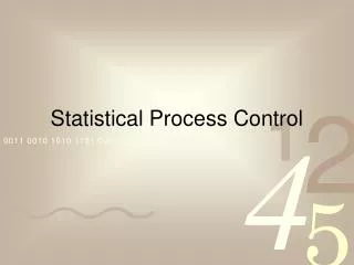
SPC (Statistical Process Control) Sample mean value 0.13% Upper control limit Normal tolerance of process 99.74% Process mean Lower control limit 0.13% 7 6 8 1 3 4 5 2 0 Sample number
Quality Control Charts Definitions • Variables Measurements on a continuous scale, such as length or weight • Attributes Integer counts of quality characteristics, such as # of good or bad • Defect A single non-conforming quality characteristic, such as a blemish • Defective A physical unit that contains one or more defects
Types of Control Charts Data monitored Chart name Sample size • Mean, range of sample variables MR-CHART 2 to 5 units • Individual variables I-CHART 1 unit • % of defective units in a sample P-CHART at least 100 units • Number of defects per unit C/U-CHART 1 or more units
Control Factors n A A2 D3 D4 d2 d3 2 2.121 1.880 0 3.267 1.128 0.853 3 1.732 1.023 0 2.574 1.693 0.888 4 1.500 0.729 0 2.282 2.059 0.880 5 1.342 0.577 0 2.114 2.316 0.864 • Control factors are used to convert the mean of sample ranges ( R ) to: (1) standard deviation estimates for individual observations, and (2) standard error estimates for means and ranges of samples For example, an estimate of the population standard deviation of individual observations (σx) is: σx = R / d2
Control Factors (cont.) • Note that control factors depend on the sample size n. • Relationships amongst control factors: A2 = 3 / (d2 x n1/2) D4 = 1 + 3 x d3/d2 D3 = 1 – 3 x d3/d2, unless the result is negative, then D3 = 0 A = 3 / n1/2 D2 = d2 + 3d3 D1 = d2 – 3d3, unless the result is negative, then D1 = 0
Mean-Range control chartMR-CHART 1. Compute the mean of sample means ( X ). 2. Compute the mean of sample ranges ( R ). 3. Set 3-std.-dev. control limits for the sample means: UCL = X + A2R LCL = X – A2R 4. Set 3-std.-dev. control limits for the sample ranges: UCL = D4R LCL = D3R
Control chart for percentage defective in a sample — P-CHART 1. Compute the mean percentage defective ( P ) for all samples: P = Total nbr. of units defective / Total nbr. of units sampled 2. Compute an individual standard error (SP ) for each sample: SP = [( P (1-P ))/n]1/2 Note: n is the sample size, not the total units sampled. If n is constant, each sample has the same standard error. 3. Set 3-std.-dev. control limits: UCL = P + 3SP LCL = P – 3SP
Control chart for individual observations — I-CHART 1. Compute the mean observation value ( X ) X = Sum of observation values / N where N is the number of observations 2. Compute moving range absolute values, starting at obs. nbr. 2: Moving range for obs. 2 = obs. 2 – obs. 1 Moving range for obs. 3 = obs. 3 – obs. 2 … Moving range for obs. N = obs. N – obs. N – 1 3. Compute the mean of the moving ranges ( R ): R = Sum of the moving ranges / N – 1
Control chart for individual observations — I-CHART (cont.) 4. Estimate the population standard deviation (σX): σX = R / d2 Note: Sample size is always 2, so d2 = 1.128. 5. Set 3-std.-dev. control limits: UCL = X + 3σX LCL = X – 3σX
Control chart for number of defects per unit — C/U-CHART 1. Compute the mean nbr. of defects per unit ( C ) for all samples: C = Total nbr. of defects observed / Total nbr. of units sampled 2. Compute an individual standard error for each sample: SC = ( C / n)1/2 Note: n is the sample size, not the total units sampled. If n is constant, each sample has the same standard error. 3. Set 3-std.-dev. control limits: UCL = C + 3SC LCL = C – 3SC Notes: ● If the sample size is constant, the chart is a C-CHART. ● If the sample size varies, the chart is a U-CHART. ● Computations are the same in either case.
SPC & Cost of Quality • Deming (Promoted SPC in Japan): • The cause of poor quality is the system, not the employee • Mgmt is responsible to correct poor quality • Juran (“Cost of Quality”: Emphasized need for accurate and complete identification of the costs of quality) : • Quality means fitness for use • Quality begins in knowing what customers want, planning processes which are capable of producing the required level of quality
From Quality to Quality Assurance Changing emphasis from “Quality” to “Quality Assurance”(Prevent defects rather than finding them after they occur) • New techniques for Quality Improvement (eg: TQM, Six Sigma): • New quality programs (Provide objective measures of quality for use of customers, SC partners, etc.) • Baldridge Award • ISO 9000/14000 Certification • Industry-specific programs (eg: TL9000(Telecom))
Correlation: x Strong positive Positive x x x Negative x x Strong negative * Source: Based on John R. Hauser and Don Clausing, “The House of Quality,” Harvard Business Review, May-June 1988. Competitive evaluation Engineering characteristics Acoustic trans., window Energy needed to open door Check force on level ground Energy needed to close door x Water resistance = Us Door seal resistance Importance to customer = Comp. A A = Comp. B B Customer requirements (5 is best) 1 2 3 4 5 x Easy to close 7 AB Stays open on a hill x AB 5 Easy to open 3 AB x x Doesn’t leak in rain 3 B A x No road noise 2 B A Importance weighting 3 2 10 9 6 6 Relationships: Strong = 9 Medium = 3 Target values Reduce energy level to 7.5 ft/lb Reduce energy to 7.5 ft/lb Small = 1 Maintain current level Maintain current level Maintain current level Reduce force to 9 lb. 5 BA B BA x x A 4 B B B x Technical evaluation (5 is best) A x 3 A x 2 A x 1
Taguchi analysis Loss function L(x) = k(x-T)2 where x = any individual value of the quality characteristic T = target quality value k = constant = L(x) / (x-T)2 Average or expected loss, variance known E[L(x)] = k(σ2 + D2) where σ2 = Variance of quality characteristic D2 = ( x – T)2 Note: x is the mean quality characteristic. D2 is zero if the mean equals the target.
Taguchi analysis (cont.) Average or expected loss, variance unkown E[L(x)] = k[Σ ( x – T)2 / n] When smaller is better (e.g., percent of impurities) L(x) = kx2 When larger is better (e.g., product life) L(x) = k (1/x2)
TQM • Total Quality Management: A philosophy that involves everyone in an organization in a continual effort to improve quality and achieve customer satisfaction. • The TQM Approach: • Find out what the customer wants • Design a product or service that meets or exceeds customer wants • Design processes that facilitates doing the job right the first time • Keep track of results • Extend quality initiatives to include suppliers & distributors.
Elements of TQM • Continual improvement • Competitive benchmarking • Employee empowerment (eg: Quality circles, etc.) • Team approach • Decisions based on facts • Knowledge of tools • Supplier quality • Identify and use quality champion • Develop quality at the source • Include suppliers
Criticism of TQM • Criticisms of TQM include: • Blind pursuit of TQM programs • Programs may not be linked to strategies • Quality-related decisions may not be tied to market performance • Failure to carefully plan the program
Obstacles to Implementing TQM • Poor inter-organizational communication • View of quality as a “quick fix” • Emphasis on short-term financial results • Internal political and “turf” wars • Lack of: • Company-wide definition of quality • Strategic plan for change • Customer focus • Real employee empowerment • Strong motivation • Time to devote to quality initiatives • Leadership
Six Sigma • Six Sigma (eg: Jack Welch @ GE): • Statistically: Having no more than 3.4 defects per million • Conceptually: A program designed to reduce defects
Six Sigma programs • Improve quality, save time & cut costs • Are employed in a wide variety of areas (Design, Production, Service, Inventory , Management, Delivery) • Focus on management as well as on the technical component • Requires specific tools & techniques • Require commitment & active participation by sr management to: • Provide strong leadership • Define performance metrics • Select projects likely to succeed
Six Sigma Programs Select and train appropriate people • The team includes top management & program champions as well as master “black belts”, “Black belts” & “Green belts” • A methodical, five- step process: Define, Measure, Analyze, Improve, Control (DMAIC)
Process Capability Analysis 1. Compute the mean of sample means ( X ). 2. Compute the mean of sample ranges ( R ). 3. Estimate the population standard deviation (σx): σx = R / d2 4. Estimate the natural tolerance of the process: Natural tolerance = 6σx 5. Determine the specification limits: USL = Upper specification limit LSL = Lower specification limit
Process capability analysis (cont.) 6. Compute capability indices: Process capability potential Cp = (USL – LSL) / 6σx Upper capability index CpU = (USL – X ) / 3σx Lower capability index CpL = ( X – LSL) / 3σx Process capability index Cpk = Minimum (CpU, CpL)
Multiplicative seasonality The seasonal index is the expected ratio of actual data to the average for the year. Actual data / Index = Seasonally adjusted data Seasonally adjusted data x Index = Actual data
Multiplicative seasonal adjustment 1. Compute moving average based on length of seasonality (4 quarters or 12 months). 2. Divide actual data by corresponding moving average. 3. Average ratios to eliminate randomness. 4. Compute normalization factor to adjust mean ratios so they sum to 4 (quarterly data) or 12 (monthly data). 5. Multiply mean ratios by normalization factor to get final seasonal indexes. 6. Deseasonalize data by dividing by the seasonal index. 7. Forecast deseasonalized data. 8. Seasonalize forecasts from step 7 to get final forecasts.
Additive seasonality The seasonal index is the expected difference between actual data and the average for the year. Actual data - Index = Seasonally adjusted data Seasonally adjusted data + Index = Actual data
Additive seasonal adjustment 1. Compute moving average based on length of seasonality (4 quarters or 12 months). 2. Compute differences: Actual data - moving average. 3. Average differences to eliminate randomness. 4. Compute normalization factor to adjust mean differences so they sum to zero. 5. Compute final indexes: Mean difference – normalization factor. 6. Deseasonalize data: Actual data – seasonal index. 7. Forecast deseasonalized data. 8. Seasonalize forecasts from step 7 to get final forecasts.
How to start up a control chart system 1. Identify quality characteristics. 2. Choose a quality indicator. 3. Choose the type of chart. 4. Decide when to sample. 5. Choose a sample size. 6. Collect representative data. 7. If data are seasonal, perform seasonal adjustment. 8. Graph the data and adjust for outliers.
How to start up a control chart system (cont.) 9. Compute control limits 10. Investigate and adjust special-cause variation. 11. Divide data into two samples and test stability of limits. 12. If data are variables, perform a process capability study: a. Estimate the population standard deviation. b. Estimate natural tolerance. c. Compute process capability indices. d. Check individual observations against specifications. 13. Return to step 1.
Quick reference to quality formulas • Control factors n A A2 D3 D4 d2 d3 2 2.121 1.880 0 3.267 1.128 0.853 3 1.732 1.023 0 2.574 1.693 0.888 4 1.500 0.729 0 2.282 2.059 0.880 5 1.342 0.577 0 2.114 2.316 0.864 • Process capability analysis σx = R / d2 Cp = (USL – LSL) / 6σx CpU = (USL – X ) / 3σx CpL = ( X – LSL) / 3σx Cpk = Minimum (CpU, CpL)
Quick reference to quality formulas (cont.) • Means and ranges UCL = X + A2R UCL = D4R LCL = X – A2R LCL = D3R • Percentage defective in a sample SP = [( P (1-P ))/n]1/2 UCL = P + 3SP LCL = P – 3SP • Individual quality observations σx = R / d2 UCL = X + 3σX LCL = X – 3σX • Number of defects per unit SC = ( C / n)1/2 UCL = C + 3SC LCL = C – 3SC