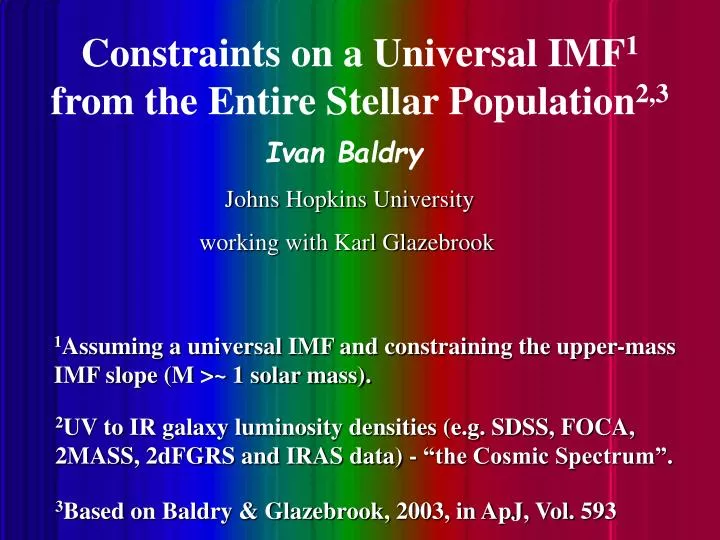
Constraints on a Universal IMF 1 from the Entire Stellar Population 2,3

1. Constraints on a Universal IMF1 from the Entire Stellar Population2,3 Ivan Baldry Johns Hopkins University working with Karl Glazebrook 1Assuming a universal IMF and constraining the upper-mass IMF slope (M >~ 1 solar mass). 2UV to IR galaxy luminosity densities (e.g. SDSS, FOCA, 2MASS, 2dFGRS and IRAS data) - “the Cosmic Spectrum”. 3Based on Baldry & Glazebrook, 2003, in ApJ, Vol. 593

2. Integrated Stellar Populations • Extragalactic astronomers fit population synthesis models to colors or spectra of galaxies to gain insights into star formation history, dust content, etc. • Usually a stellar initial mass function (IMF) is assumed because of the age-IMF degeneracy. • This age-IMF degeneracy can be broken for the Universe as a whole (assuming the Copernican principle): • Age = 13.70.2 Gyr (Spergel et al. 2003); • Meas. of cosmic star formation history (Madau et al. 1996, `98); • Meas. of the local “cosmic spectrum” (Baldry et al. 2002).

3. Overview of Fitting • Stellar initial mass function (IMF) • Cosmic star formation history (SFR tracers 0 < z < ~5) • Chemical evolution • Dust attenuation • Population synthesis models • DATA – luminosity densities (0 < z < 0.2): • FOCA (balloon), 0.2 microns (Sullivan et al. 2000); • SDSSugriz, 0.3-1 microns (Blanton et al. 2003); • 2MASS, 2 microns, with z (Cole et al., Kochanek et al. 2001); • H-alpha, attenuation-corrected (Gallego et al. 1995 and others); • IRAS FIR (Saunders et al. 1990) converted to total dust emission.

4. Stellar IMF Parameterization Note unusual y-axis scaling: mass fraction m–0.5 for 0.1 < m < 0.5 m–Gfor 0.5 < m < 120 nlog m G=1.35 is Salpeter slope

5. Cosmic Star Formation History REDSHIFT “Madau plot” versus time Various measurements, e.g, Lilly et al. 1996, Madau et al. 1996/98, Cowie et al. 1999, Steidel et al. 1999, Lanzetta et al. 2002, + more. SFR  (1+z)b for z<1 (0.5 < b < 4.0 allowed) and, SFR  (1+z)a for 1<z<5 (SFR = 0 for z>5; meet at z=1).

6. Cosmic Chemical Evolution The cosmic stellar-mass weighted metallicity is approx. solar (cf. our neighborhood in the Milky Way). Compare ‘closed box’ with ‘constant metallicity’ approximations. Allow average Z from about 0.5 Zsolar to 2 Zsolar.

7. Cosmic Dust Attenuation Law Inclination-averaged attenuations. Compilation from Calzetti (2001). Estimated dust attenuation allowing for different contributionsfrom late- and early-type galaxies as a function of wavelength. About 90% of the luminosity density is derived from late type galaxies at 0.2 microns and about 50% at visible to near-IR wavelengths. Power-law with exponent ~ –0.8

8. Population Synthesis • PEGASE.2 (Fioc & Rocca-Volmerange 1997, 1999): • Covers UV to IR; • Includes stellar and nebular (continuum and line emission); • Can specify arbitrary power law IMFs and SFH. • Evolutionary tracks from Padova group. • Theoretical spectra from Clegg & Middlemass (1987) and Lejeune et al. (1997) (derived from Kurucz models, NextGen and Fluks catalogues). • From the output spectra, determine: • Colors through FOCA, SDSS and 2MASS filters; • Total dust emission for various dust power laws; • H-alpha luminosity (reprocessed Lyman continuum emission).

9. Data Summary Local Luminosity Density Measurements from Various Surveys (0<z<0.2)

10. Effect of Various Parameters Normalized at 0.56 microns. DATA FOCA, Sullivan et al. 2000 SDSS, Blanton et al. 2003 2MASS, Cole et al. 2001, Kochanek et al. Hawaii, Huang et al. 2003 AB Magnitudes (a log fn) Wavelength (0.15-2.5 microns)

11. Results Assuming: constant SFR from z = 1 to 5, average metallicity = solar. Fitting to 0.20, 0.32, 0.42, 0.56, 0.68, 0.81, 2.2 + Ha + dust emission. Red contours for constant Z Blue contours for closed box approx. redshift < 1 star formation power law (Salpeter = 1.35) Dc2=(1, 2.3, 6.2, 11.2)

12. Results continued Assuming: high z>1 SFR a (1+z)2, average metallicity = solar. Fitting to 0.2-0.8, 2.2 + Ha + total dust emission. Red contours for constant Z Blue contours for closed box approx. redshift < 1 star formation power law (Salpeter = 1.35) Dc2=(1, 2.3, 6.2, 11.8)

13. Results continued • G=1.1±0.2 marginalized over dust, SFH, 0.5<Z/Zsolar<2. • Scalo IMF is inconsistent with data and models (cf. Madau, Pozzetti & Dickinson 1998 and Kennicutt, Tamblyn & Congdon 1994 [incl. Ha EWs]). • Stellar mass density of the Universe is in the range 0.15% to 0.28% (0.12% to 0.35% with low-mass IMF uncertainty, or 3% to 8% of baryon density). • Stellar bolometric emission is (1.7-2.4) x 1035 W Mpc-3 and dust emission is (0.4-1.0) x 1035, which implies a modest effective average attenuation in the ultraviolet of A2000 < ~60% (< ~1 mag). • CAVEAT – results rely on accuracy of population synthesis…

14. Local Luminosity Densities bolometric luminosity per log l bin Data and best-fit model spectrum: the stellar and the HIIregion gas emission (Fioc & Rocca-Volmerange) and; the dust emission (Dale & Helou). AGN contribution not shown.

15. Future and Current Surveys • Local imaging surveys (z~0.1): • (SDSS has set the bench mark, >105 galaxies with redshifts and ugriz photometry, >103 deg2) – optical; • GALEX all-sky survey – ultraviolet; • VISTA – near-infrared (also 2MASS with 6dFGS redshifts); • ASTRO-F – mid- to far-infrared. • Deeper imaging surveys: • GALEX deep surveys – ultraviolet; • HST – ACS, NICMOS – optical, near-IR; • SIRTF – mid- to far-infrared.

16. … Extra slides follow.

17. Cosmic Star Formation History • Meas. of comoving star-formation rate density (MO/yr/Mpc3) as a function of redshift (or time). CSFH analysis removes uncertainties associated with dynamical history, i.e. consider the Universe to be a single average galaxy. Determine SFR per comoving volume: (modulo dust, SB, etc… corrections) Luv, LFIR, L700Mhz LHa, LHb, L[OII] Number of massive stars formed / unit time

18. Madau, Pozetti & Dickinson 1998 Fig 3: Salpeter IMF; SMC-type dust in a foreground screen; E(B–V)=0.1. 2.2 mm 1.0 mm .44 mm .28 mm .15 mm

19. Madau, Pozetti & Dickinson 1998 2.2 mm 1.0 mm .44 mm .28 mm .15 mm Salpeter IMF, E(B–V) = 0.011(1+z)2.2 Scalo IMF, no dust

20. Table of IMF Comparisons