Download
1 / 40
400 likes | 514 Views
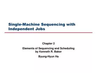
Single-Machine Sequencing with Independent Jobs. Chapter 2 Elements of Sequencing and Scheduling by Kenneth R. Baker Byung-Hyun Ha. Outline. Introduction Preliminaries Problem without due dates: elementary results Flowtime and inventory Minimizing total flowtime

E N D
Single-Machine Sequencing with Independent Jobs Chapter 2 Elements of Sequencing and Schedulingby Kenneth R. Baker Byung-Hyun Ha
Outline • Introduction • Preliminaries • Problem without due dates: elementary results • Flowtime and inventory • Minimizing total flowtime • Minimizing total flowtime: the weighed version • Problem with due dates: elementary results • Lateness criteria • Minimizing the number of tardy jobs • Minimizing total tardiness • Due dates as decisions • Summary
Introduction • Pure sequencing problem • Specialized scheduling problem in which an ordering of jobs completely determines a schedule • Single-machine problem • Simplest pure sequencing problem, but important • Reveals a variety of scheduling topics in a tractable model • A context in which to investigate many performance measures and solution techniques • A building block in the development of a comprehensive understanding of scheduling concepts • A way to complex problems • Single-machine problems as a part of complex ones • Solving imbedded single-machine problems and incorporating the results into larger problems • Bottleneck analysis in multiple-operation processes • Decisions using resources as aggregated one
Introduction • Characteristics of basic single-machine problem C1. A set of n independent, single-operation jobs is available for processing simultaneously (at time zero) C2. Setup times for the jobs are independent of job sequence and are included in processing times C3. Job descriptors are deterministic and known in advance C4. One machine is continuously available and never kept idle while work is waiting C5. Once an operation begins, it proceeds without interruption (i.e. no preemption is allowed)
Introduction • Permutation schedule • Sequence of n jobs permutation of job indices 1, 2, ..., n • Single-machine problem pure sequencing problem • A schedules can be completely specified by a permutation of integers • Total # of distinct schedule – n! • Indication of position in sequence using brackets • [5] = 2 5th job in sequence is job 2 • d[1] due date of 1st job in sequence
Preliminaries • Job descriptors • Input to scheduling problem • Examples • pj -- processing time • Amount of processing required by job j pj will generally include both processing time and facility setup time under C2 • rj -- ready time • Time at which job j is ready (or available) for processing • rj can be regarded as arrival time, but rj = 0 under C1 • dj -- due date • Time at which processing of job j is due to be completed
Preliminaries • Information for evaluating schedule • Output from scheduling • Examples • Cj -- completion time • Time at which processing of job j is finished • Fj -- flowtime • Time job j spends in system; Fj= Cj– rj • Response of system to individual demands for service (turnaround time) • Lj -- lateness • Amount of time by which completion time of job j exceeds its due date;Lj = Cj – dj • Conformity of schedule to given due date • Negative value whenever job is completed early • Tj -- tardiness • Lj if job j fail to meet its due date, 0 otherwise; Tj = max{0, Lj} • Uj -- unit penalty • Uj = 1, if Cjdj; 0, otherwise
Preliminaries • Due date related penalty functions Lj Tj dj Cj dj Cj Uj 1 dj Cj
Preliminaries • Performance measures • 1-dimensional aggregated quantities about all jobs • Used generally for evaluation of schedules • Functions of set of completion time in schedule, usually • Z = f(C1, C2, ..., Cn) • Examples • Total flowtime -- F = j=1nFj • Total tardiness --T = j=1nTj • Maximum flowtime--Fmax = max1jn{Fj} • Maximum tardiness--Tmax = max1jn{Tj} • Number of tardy jobs, or total unit penalty--U = j=1nUj • Mean flowtime, mean tardiness, proportion of tardy jobs • Problem description • F-problem -- minimization of total flowtime • T-problem • Cmax-problem
Preliminaries • Regular measures • Performance measure Z is regular, if (a) scheduling object is to minimize Z, and (b) Z can increase only if at least one of the completion times in schedule increases (b) Z' Z Cj' Cj for some job j, where Z = f(C1, C2, ..., Cn) is value of a measure of schedule S and Z' = f(C1', C2', ..., Cn') is value of the same measure of some different schedule S' (b) Cj' Cj for all job j Z' Z , where ... • Measures that presented in the previous slide are all regular
Preliminaries • Dominant set • A set of schedules is dominant if it is sufficient to be considered for finding solution • Reduced search space from complete enumeration • Verification of dominant set D of schedules for regular measures 1. Consider an arbitrary schedule S (which contains completion times Cj) that excluded from D 2. Show that there exists a schedule S' in D, in which Cj' Cj for all j 3. Therefore Z' Z for any regular measure, and so S' is at least as good as S 4. Hence, in searching for an optimal schedule, it is sufficient to consider only schedules in D • Dominant sets for regular measures in basic single-machine problems • Set of permutation schedules (without preemption) C5 could be relaxed • Set of schedules without idle time C4 could be relaxed
Preliminaries • Theorem 1 • In the basic single-machine problem, schedule without inserted idle time constitute a dominant set. • Proof sketch of Theorem 1 • Suppose schedule S by which machine is idle during interval (a, b). • There exists schedule S' such that Cj' = Cj, if Cj a; Cj' = Cj – (b – a), otherwise. • Cj' Cj for all j. Hence, Z' Z for any regular measure. • Therefore, schedules without idle time constitute a dominant set. • Theorem 2 • In the basic single-machine problem, schedules without preemption constitute a dominant set. • HOMEWORK #1 • Prove Theorem 2 RIGOROUSLY
Problem without Due Dates: Elementary Results • Flowtime and inventory • Minimizing total flowtime • Minimizing total flowtime: the weighed version
Flowtime and Inventory • Two closely related objectives • Rapid turnaround of customers -- minimizing total flowtime • Low inventory levels -- minimizing average # of jobs in system • Notations • J(t) -- number of jobs in system at time t, J -- time average of J(t) • Fmax = p1 + p2 + ... + pn -- makespan J(t) J(t) n n n – 1 n – 1 n – 2 n – 2 2 2 1 1 p[1] p[2] p[3] ... p[n-1] p[n] t p[1] p[2] p[3] ... p[n-1] p[n] t A = np[1] + (n – 1)p[2] + ... + 2p[n-1] + p[n] A = JFmax = F F = F[1] + F[2] + ... + F[n]
Flowtime and Inventory • Relationship between flowtime and inventory • J= F/Fmax -- J is directly proportional to F • The relationship extends well beyond single-machine problem • In dynamic environment where jobs arrive over time • In infinite-horizon models where new work arrives continuously • In probabilistic systems where process times are uncertain • Little’s law • L = W, where • L -- long-term average number of customers in a stable system -- long-term average arrival rate W -- long-term average time a customer spends in the system
Minimizing Total Flowtime • Equivalent problem to F-problem • Minimizing the area under J(t) function • Using shortest processing time (SPT) sequencing • Sequencing jobs in nondecreasing order of processing times J(t) n n – 1 n – 2 2 1 p[1] p[2] p[3] ... p[n-1] p[n] t
Minimizing Total Flowtime • Theorem 3 • Total flowtime is minimized by Shortest Processing Time (SPT) sequencing (p[1] p[2] ... p[n]). • Proof sketch of Theorem 3 (proof by contradiction) • Suppose there is a sequence S that is optimal but not SPT sequence. • In S, there exists a pair of adjacent jobs, i and j, with j following i, such that pi pj . • Construct sequence S' in which job i and j are interchanged. • Fi + Fj Fj' + Fi' implies that F F', which is a contradiction. • Therefore, for all S, if S is optimal, then S is SPT sequence. S ... ... i j Fi Fj S' ... ... j i Fi' Fj'
Minimizing Total Flowtime • Proof by contradiction • Method 1. Suppose the statement to be proved is false. That is, suppose that the negation of the statement is true. 2. Show that this supposition leads logically to a contradiction. 3. Conclude that the statement to be proved is true Exercise: prove that there is no greatest integer • Suppose not. That is, suppose there is a greatest integer N. • Then, N n for every integer n. • Let M = N + 1. • M is an integer since it is a sum of integers. • M N since M = N + 1. • So N is not the greatest integer, which is a contradiction.
Minimizing Total Flowtime • Theorem 3, revisited • Predicates • O(S) -- S is optimal, SPT(S) -- S is SPT sequence • Definitions • S, O(S) (S', F F') S, O(S) (S', F F') --- • Theorem 3 • S, O(S) SPT(S) • Negation of Theorem 3 • (S, O(S) SPT(S)) (S, O(S) SPT(S)) S, O(S) SPT(S) • Proof of Theorem 3 by contradiction • Suppose not. That is, suppose there is S such that not SPT(S) but O(S). • Then, S', F F' by . • In S, there exists a pair of adjacent jobs, i and j, with j following i, such that pi pj . • Let S' be the same sequence with S except job i and j are interchanged. • F F' since Fi + Fj Fj' + Fi'. • So S is not optimal by , which is a contradiction.
Minimizing Total Flowtime • Proof of Theorem 3 by construction 1. Begin with any non-SPT sequence 2. Find a pair of adjacent jobs i and j, with j following i, such that pi pj . 3. Interchange jobs i and j in sequence 4. Return to Step 2 iteratively, improving the performance measure each time, until eventually the SPT sequence is constructed. • Another perspective of Theorem 3 • Total flowtime as scalar product of two vectors • j=1nFj = j=1n i=1jp[i] = j=1n(n – j + 1)p[j] • Solution of minimizing such a scalar product • One sequence with nonincreasing, the other with nondecreasing • Since one is already nonincreasing, the other should be nondecreasing
Minimizing Total Flowtime • Related properties with Theorem 3 • SPT sequencing minimizes J as well as F • If waiting time of job j is defined as its time spent in system prior to the start of its processing, SPT minimizes total waiting time. • SPT minimizes the maximum waiting time
Minimizing Total Flowtime: Weighted Version • Flowtime and inventory • Fw = j=1nwjFj-- total weighted flowtime • V(t) -- total value of inventory in the system at time t • V -- time average of V(t) • A = j=1n p[j] i=jn w[i] = VFmax = Fw = j=1nwjFj • Sequence which minimizes one will minimize the other V(t) wj w[n] + w[n-1] w[n] ... t p[1] p[2] p[3] p[n-1] p[n]
Minimizing Total Flowtime: Weighted Version • Theorem 4 • Total weighted flowtime is minimized by Shortest Weighted Processing Time (SWPT) sequencing (p[1]/w[1] p[2]/w[2] ... p[n]/w[n]). • HOMEWORK #2 • Prove Theorem 4
Problem with Due Dates: Elementary Results • Lateness criteria • Minimizing the number of tardy jobs • Minimizing total tardiness • Due dates as decisions
Lateness Criteria • Total lateness and maximum lateness • Assuming 3 jobs {1, 2, 3} • p1 = 5, p2 = 2, p3 = 3 • d1 = 6, d2 = 4, d3 = 8 • r1 = r2 = r3 = 0 • Sequencing • (2, 1, 3) • Lateness (Cj – dj) • C[1] = 2, C[2] = 7, C[3] = 10, d[1] = 4, d[2] = 6, d[3] = 8 • L[1] = 2 – 4 = –2, L[2] = 7 – 6 = 1, L[3] = 10 – 8 = 2 • L = 1, Lmax = 2 • Theorem 5 • Total lateness is minimized by SPT sequencing. • Proof sketch of Theorem 5 • L = j=1nLj = j=1n(Cj – dj) = j=1n(Fj – dj) = j=1nFj – j=1ndj . 2 1 3 2 7 10
Lateness Criteria • Theorem 6 • Maximum lateness and maximum tardiness are minimized by Earliest Due Date (EDD) sequencing (d[1] d[2] ... d[n]). • Proof sketch of Theorem 6 • Similar to proof of Theorem 3, we employ adjacent pairwise interchange of two adjacient jobs i and j, where dj di but Ci Cj . • max{Li, Lj} max{Li', Lj'} Lmax of S Lmax of S' S S S ... ... ... ... ... ... i j i j i j Li Li Lj di Ci Ci di dj Cj Lj Lj Li dj Cj dj Cj Ci di S' S' S' ... ... ... ... ... ... j i j i j i Lj' Lj' dj Cj' dj Cj' Lj' Li' Li' Li' di Ci' di Ci' Cj' dj Ci' di
Lateness Criteria • Another measure of urgency • Slack time -- sj= dj– t – pj • Longest job is most urgent • Minimum slack time (MST) sequencing • d[1] – p[1] d[2] – p[2] ... d[n] – p[n] • Theorem 7 • Among schedules with no idle time, the minimum jobs lateness is maximized by MST sequencing
Minimizing the Number of Tardy Jobs • U-problem and EDD • EDD is optimal sequence if there is no tardy job (U = 0) • EDD is also optimal if there is only one tardy job • EDD may not be optimal if there are more than one tardy jobs ... ... i j k l m dk dj dl di dm ... ... i j di dj
Minimizing the Number of Tardy Jobs • Optimal sequence form of U-problem • Set B of early jobs and set A of late jobs • Algorithm 1 (Minimizing U) 1. Index jobs using EDD order and place all jobs in B. A = . 2. If no jobs in B are late, stop. Otherwise, identify the first late job j[k] in B. 3. Identify the longest job among the first k jobs in sequence. Remove this job from B and place it in A. Return to Step 2. B A ... ... Early jobs Late jobs ... ... ... longest [k-1] d[k-1] d[k]
Minimizing the Number of Tardy Jobs • Proof of Optimality of Algorithm 1 • See Pinedo, 2008, p. 48. • Exercise • Get optimal sequence which minimize U. • Weighted version of U-problem • NP-hard, i.e., as difficult as, or even more difficult than, NP-Complete
Minimizing Total Tardiness • Minimization of total tardiness • Quantification of qualitative goal of meeting job due dates • Time-dependent penalties on late jobs, no benefits from completing jobs early • Difficulties • Tardiness is not a linear function of completion time • NP-hard problem • First simple and possible analysis • Consider only two adjacent jobs, i and j, and figure out the appropriate order of decreasing total tardiness • Let • Tij = Ti(S) + Tj(S) = max{p(B) + pi – di, 0} + max{p(B) + pi + pj – dj, 0} • Tji = Tj(S') + Ti(S') = max{p(B) + pj – dj, 0} + max{p(B) + pi + pj – di, 0} B A B A S S' ... ... ... ... i j j i p(B) p(B)
Minimizing Total Tardiness • Agreeability • Two set of parameters, uj and vjare agreeable if ui ujimplies vi vj • Case 1: agreeable processing time and due dates (pi pj, di dj) • Remember • Tij = max{p(B) + pi – di, 0} + max{p(B) + pi + pj – dj, 0} • Tji = max{p(B) + pj – dj, 0} + max{p(B) + pi + pj – di, 0} • Case 1.1: p(B) + pi di • Tij = max{p(B) + pi + pj – dj, 0} • Case 1.1.1: p(B) + pjdj , p(B) + pi + pjdi • Tji = max{p(B) + pi + pj – di, 0} max{p(B) + pi + pj – dj, 0} = Tij • Case 1.1.2: p(B) + pjdj , p(B) + pi + pjdi • Tji = max{p(B) + pj – dj, 0} max{p(B) + pi + pj – dj, 0} = Tij • Case 1.1.3: p(B) + pjdj , p(B) + pi + pjdi • Tij – Tji = (p(B) + pi + pj – dj) – (p(B) + pj – dj) – (p(B) + pi + pj – di) = –p(B) – pj + di –p(B) – pi + di 0 • Therefore, Case 1.1 yield TijTji , so it is preferable that job j precede job i.
Minimizing Total Tardiness • Case 1: pi pj, di dj (cont’d) • Remember • Tij = max{p(B) + pi – di, 0} + max{p(B) + pi + pj – dj, 0} • Tji = max{p(B) + pj – dj, 0} + max{p(B) + pi + pj – di, 0} • Case 1.2: p(B) + pi di • Tij = p(B) + pi – dj + p(B) + pi + pj – dj • Tji = max{p(B) + pj – dj, 0} + p(B) + pi + pj – di • Tij – Tji = p(B) + pi – dj – max{p(B) + pj – dj, 0} • Case 1.2.1: p(B) + pjdj • Tij – Tji = p(B) + pi – dj p(B) + pi – di 0 • Case 1.2.2: p(B) + pjdi • Tij – Tji = p(B) + pi – dj – (p(B) + pj – dj) = pi – pj 0 • Therefore, Case 1.2 yield TijTji , so it is preferable that job j precede job i. • Theorem 8 • For any pair of jobs, suppose that processing times and due dates are agreeable. Then total tardiness (T) is minimized by SPT (or, equivalently, EDD) sequencing.
Minimizing Total Tardiness • Case 2: parameters are not agreeable (pi pj, di dj) • Remember • Tij = max{p(B) + pi – di, 0} + max{p(B) + pi + pj – dj, 0} • Tji = max{p(B) + pj – dj, 0} + max{p(B) + pi + pj – di, 0} • Case 2.1: p(B) + pidi • Tji = max{p(B) + pi + pj – di, 0} max{p(B) + pi + pj – dj, 0} = Tij • Therefore, Case 2.1 yield TjiTij , so it is preferable that job i (with earlier due date) precede job j. • Case 2.2: p(B) + pidi • Case 2.2.1: p(B) + pi + pjdj • Tij = p(B) + pi – di • Tji = p(B) + pi + pj – diTij • Therefore, Case 2.2.1 yields TjiTij, so it preferable that job i (with earlier due date) precede job j.
Minimizing Total Tardiness • Case 2: (pi pj, di dj) (cont’d) • Remember • Tij = max{p(B) + pi – di, 0} + max{p(B) + pi + pj – dj, 0} • Tji = max{p(B) + pj – dj, 0} + max{p(B) + pi + pj – di, 0} • Case 2.2: p(B) + pidi (cont’d) • Case 2.2.2: p(B) + pi + pjdj • Case 2.2.2.1: p(B) + pjdj • Tij = p(B) + pi – di + p(B) + pi + pj – dj • Tji = p(B) + pi + pj – di • Tij – Tji = p(B) + pi – dj • Therefore, Case 2.2.2.1 yields that it is preferable that job i precede job j unless p(B) + pidj , where job j (shorter job) may precede job i. • Case 2.2.2.2: p(B) + pjdj • Tij = p(B) + pi – di + p(B) + pi + pj – dj • Tji = p(B) + pj – dj + p(B) + pi + pj – di • Tij – Tji = pi – pj 0 • Therefore, Case 2.2.2.2 yield TijTji , so it is preferable that job j (shorter job) precede job i.
Minimizing Total Tardiness • Theorem 9 • In case of T-problem, if jobs i and j are the candidates to begin at time t, then the job with earlier due date should come first, except ift + max{pi, pj} max{di, dj},in which case the shorter job should come first. Combined results from Case 1 and Case 2 • Review of Theorem 9 • Outcome depends on time t when candidate jobs are compared • Not sufficient but necessary condition of T-problem • It does not tell whether job i and j should come early or late in schedule • Consider following T-problem • Check schedule (2, 1, 3) • Check optimal schedule (1, 3, 2)
Minimizing Total Tardiness • Modified due date (MDD) • dj' = max{dj, t + pj} • MDD priority rule • If jobs i and j are the candidates to begin at time t, then the job with the earlier modified due date should come first. • MDD priority rule is consistent with Theorem 9. • HOMEWORK #3 • Prove MDD priority rule is consistent with Theorem 9. • Hint: divide into cases and conquer, e.g., Case 1: agreeable, i.e., pi pj, di dj : t + max{pi, pj} = t + pj, max{di, dj} = dj Case 1.1: t + pj dj jobi comes first according to Theorem 9 dj' = max{dj, t + pj} = t + pj Case 1.1.1: di t + pi di' = max{di, t + pi} = di dj t + pj = dj' job i comes first from the rule Case 1.1.2: ...
Minimizing Total Tardiness • Specialized results for T-problem • If EDD sequence produces no more than one tardy job, it is optimal. • If all jobs have the same due dates, T is minimized by SPT sequencing. • If it is impossible for any job to be on time in any sequence, T is minimized by SPT sequencing. • If SPT sequencing yields no jobs on time, it minimizes T.
Due Date as Decisions • Due date as a matter of negotiation • In practice • Reasonable models would introduce much more complexity • A simple step, here • Treating due date as a decision variable, subject to some constraints • Environment • Due date can be selected at job’s arrival time (rj) • Selection of due date depends only on information about the job itself • Possible rules selecting due date • CON -- constant flow allowance: dj = rj + • SLK -- equal slack flow allowance: dj = rj + pj + • TWK -- total work flow allowance: dj = rj + pj • Some results • CON due dates are dominated by either SLK or TWK due dates • TWK will tend to be the best rule most of time
Summary • Basic single-machine model • Fundamental in the study of sequencing and scheduling • Scheduling objectives • Solution strategies • Using simple sequencing rules, such as SPT and EDD • Using more intricate construction for U-problem • We could not solve T-problem