Understanding Histograms and Data Visualization in Quantitative Analysis
In this chapter, we explore the vast landscape of data visualization, emphasizing the importance of choosing the right type of chart for quantitative data. Unlike bar charts that are suitable for categorical data, histograms offer a visually effective way to represent quantitative data distributions. We will dive into the significance of frequency tables, highlighting the key differences between histograms and other chart types, such as stem-and-leaf plots and time plots. Additionally, we will discuss how to accurately describe data distributions by assessing shape, center, and spread.


Understanding Histograms and Data Visualization in Quantitative Analysis
E N D
Presentation Transcript
More Chapter 3! (or Chapter 4)
Brave New Data • We are no longer limited to charts which only work for categorical data. • We have three more charts at our disposal. • Even though I do not think the book stresses this enough, frequency tables and relative frequency tables are still useful for quantitative data. • Bar charts and pie charts, however, are not.
Just Kidding On The Bar Charts • We do not use bar charts (or column charts) for quantitative data. • We use histograms. • These are, as you can hopefully see, charts with bars. • Doesn’t that make them bar charts?
It Totally Should • Distinguishing between histograms and bar charts borders on obnoxiousness. • However, it is important to note that bar charts have gaps and histograms do not, and so we call them something different. • The primary purpose in the distinction is help reinforce that categorical data and quantitative data are different.
What Makes Histograms Special • Bar charts can show data in whatever order they like, but histograms need to go in order. • Since they are used with quantitative data, the order is built in. • If there is an interval with no data, you are still expected to have it in your graph as an empty space. • A gap on a histogram means there was a gap in the data.
Categorical vs. Quantitative • Sometimes the data can be made into either. • For example, scores and letter grades can both be found for the quiz.
Histograms FTW! • In later chapters, histograms will be the preferred plot for categorical data in general. • Dotplots are a fun way to amuse yourself…if you are into making charts and graphs. • Stem-and-leaf plots are useful, but can take forever and also require intense attention to detail. • They are very convenient for displaying two distributions side by side. • While not mentioned much in this chapter, there are also lineplots, which are like histograms, except instead of bars, there is a line connecting the frequencies.
Stem-and-leaf Diagrams • Also known as stemplots. • The stem contains the beginning of each data point (such as the tens place or hundreds place). • Each data point is called a leaf. • Each leaf needs to be the same number of characters. • If you have double-digit leaves, it is wise to leave a space after each one.
Stem-and-leaf Diagrams • The stem can be broken down into partial categories, such as high and low. • The stem can be surrounded on both sides with leaves, representing two distributions side by side. • The leaves need to all take up the same space. • On a computer, the Courier font ensures that all text takes up the same space left to right.
Stem-and-leaf Diagrams • The leaves should be in numerical order within each stem. • This means sorting the data first. • No stem should be left out, which means that if you do not have any leaves for a given stem, you still need it, but it just gets left empty. • Probably best done by hand, and for relatively small data sets (like 30 subjects or less).
Timeplots • These are the only lineplots mentioned in your book. • They are the most common kind of line plot. • You basically plot the dots and connect the dots. • They are not only really straightforward, but they are also intuitive, so regular people can look at them and see trends.
Back to Histograms • Histograms should be evenly scaled. • This means even class widths. • The book would say even bin sizes. • This also can be expressed as even intervals. • Histograms should include every interval between the start and stop of the data. • Even if they are empty. • Especially if they are empty.
Describing Distributions • There are three key areas to describe when discussing a distribution. • Shape – This usually means counting the high points, checking for symmetry, and looking for extreme values. • These high points are called modes. • Center – This will usually focus on an appropriate measure of central tendency. • The Mean and the Median are common. • Spread – This will usually mean giving an indication of how spread out the data is. • The Range and the Standard Deviation are common.
Shape • Within the shape category, there are three things we will tend to focus on. • First is known as modality. That is basically just how many bumps. • One exception is a uniform distribution. • The second is symmetry and skew. • A graph is considered skewed if it leans more towards one side of the mode than the other. • The third is outliers. • Next chapter we will learn how to identify them numerically, but for now, we will only focus on outliers that are obvious.
Center • Next chapter we will learn all about calculating centers. • For now, we will just rely mostly on intuition. • If the graph is skewed in a direction, the mean will be more in that direction than in the other direction, and might not match up perfectly with the mode.
Spread • We will learn how to calculate spread. • We will learn how to calculate spread by hand even. • Once we have finished that, you will understand spread really well. • For now, it just relates to how wide the graph is.
Comparing Distributions • A good rule of thumb is that if you have two distributions, graph them separately, but on the same scale as one another. • If you fix the scales, a more accurate picture of how they match up forms. • Comparing two distributions on a stem-and-leaf diagram is a bit different. • Comparing two sets of categorical variables on the same bar chart can be handy as long as they have the same categories. • It is common for bar charts to be used in place of histograms to compare two or more sets of quantitative data. • It is worth your while to see this kind of graph.
Assignments • Chapter 3: 5, 9, 19, 25, 33, 37 • Due Monday • Chapter 4: 4, 8, 11, 17, 18, 30, 33 • Due Tuesday • Read Chapter 4. • Make time to see or e-mail me with quiz questions. • Begin studying for Chapter 4 Quiz on Monday. • So maybe do the chapter 3 homework before Sunday so you have time to study.
Quiz Bulletpoints • Be familiar with the differences between a histogram and a bar chart. • Be familiar with the advantages and disadvantages of a stem-and-leaf diagram. • Be familiar with the what-not-to-do list in chapter 4. • Be familiar with the what-not-to-do list in chapter 4. • Know when and how to transform data.
But What If I Don’t Have A Book?!?! • Me memememe. • j/k lol :) • Here’s the list: • Don’t Make a Histogram of a Categorical Variable. • Don’t Look for Shape, Center, and Spread of a Bar Chart. • Don’t Use Bars in Every Display – Save Them for Histograms and Bar Charts. • Choose a Bin Width Appropriate to the Data. • Avoid Inconsistent Scales • Label Clearly