Download
1 / 22
220 likes | 252 Views
This paper explores the use of approximate adiabatic evolution to solve NP-complete problems. It discusses the encoding of problems and solutions in the initial and final states of the system and provides examples of algorithms that can be implemented using this approach. The paper also discusses the challenges of decoherence and the need for quantum error correction. It concludes with an analysis of the advantages of adiabatic quantum computation and the potential for future research.

E N D
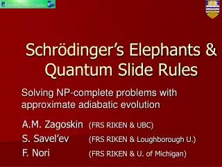
Schrödinger’s Elephants & Quantum Slide Rules Solving NP-complete problems with approximate adiabatic evolution A.M. Zagoskin (FRS RIKEN & UBC) S. Savel’ev (FRS RIKEN & Loughborough U.) F. Nori (FRS RIKEN & U. of Michigan)
Consecutive application of unitary transformations (quantum gates) Problem encoded in the initial state of the system Solution encoded in the final state of the system digital operation Examples: Shor’s algorithm Grover’s algorithm quantum Fourier transform Precise time-domain manipulations complex design and extra sources of decoherences Problem and solution encoded in fragile strongly entangled states of the system effective decoherence time must be large Quantum error-correction (to extend the coherence time of the system) overhead (threshold theorems: 104-1010(!)) Aharonov, Kitaev & Preskill, quant-ph/05102310 Standard quantum computation
Continuous adiabatic evolution of the system Problem encoded in the Hamiltonian of the system Solution encoded in the final ground state of the system Farhi et al., quant- ph/0001106; Science 292(2001)472 The approach is equivalent to the standard quantum computing Aharonov et al., quant- ph/0405098 “Space-time swap”: the time-domain structure of the algorithm is translated to the time-independent structural properties of the system Ground state is relatively robust much easier conditions on the system and its evolution Well suited for the realization by superconducting quantum circuits Kaminsky, Lloyd & Orlando, quant-ph/0403090 Grajcar, Izmalkov & Il’ichev, PRB 71(2005)144501 Adiabatic quantum computation
Travelling salesman’s problem* • N points with distances dij • Let nia=1 if i is stop #a and 0 otherwise; there are N2 variables nia (i,a = 1,…,N) • The total length of the tour *See e.g. M. Kastner, Proc. IEEE 93 (2005) 1765
Travelling salesman’s problem • The cost function
Travelling salesman’s problem • Ising Hamiltonian
Adiabaticity parameter Spin Hamiltonian
RMT theory near centre of spectrum* Diffusive behaviour Residual energy β = 1 (GOE); 2 (GUE) Simulated annealing** ζ≤ 6 Approximate adiabatic optimization vs. simulated annealing **G.E. Santoro et al., Science 295 (2002) 2427 *M. Wilkinson, PRA 41 (1990) 4645
Running time vs. residual energy • Classical/quantum simulated annealing (classical computer) • Approximate adiabatic algorithm (quantum computer)
Solution is encoded in the final ground state Error produces unusable results (excited state does not, generally, encode an approximate solution) Objective: minimize the probability of leaving the ground state Solution is a (smooth enough) function of the energy of the final ground state Error produces an approximate solution (energy of the excited state is close to the ground state energy) Objective: minimize the average drift from the ground state Relevant problems: finding the ground state energy of a spin glass traveling salesman problem AQC vs. Approximate AQC
Generic description of level evolution: Pechukas gas* *P. Pechukas, PRL 51 (1983) 943
Pechukas gas kinetics: taking into account Landau-Zener transitions
4-flux qubit register *M. Grajcar et al., PRL 96 (2006) 047006
Conclusions • Eigenvalues behaviour is not described by simple diffusion • Marginal states behaviour qualitatively different: adiabatic evolution generally robust • Analog operation of quantum adiabatic computer provides exponential speedup • Advantages of Pechukas mapping: exact, provides intuitively clear description and controllable approximations (BBGKY chain) • In future: external noise sources; mean-field theory; quantitative theory of a specific algorithm realization; investigation of the class of AA-tractable problems