Download
1 / 27
270 likes | 419 Views
Learn about RISC machines, register windows, Flynn’s taxonomy, vector processors, and vectorization concepts for optimized parallel processing. Understand the properties and components of vector processors and how vectorization boosts performance.

E N D
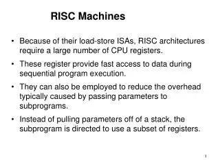
RISC Machines • Because of their load-store ISAs, RISC architectures require a large number of CPU registers. • These register provide fast access to data during sequential program execution. • They can also be employed to reduce the overhead typically caused by passing parameters to subprograms. • Instead of pulling parameters off of a stack, the subprogram is directed to use a subset of registers.
Register Windows • This technique was motivated by quantitative analysis of how procedures pass parameters back and forth • Normal parameter passing: Uses the stack • But this is slow • Would be faster to use registers • Benchmarks indicate that • Most procedures only pass a few parameters • A nesting depth of more than 5 is rare
User View of Registers • Used on SPARC
Overlap Register Windows CWP = Current Window Pointer
Register Windows • Parameters are “passed” by simply updating the window pointer • All parameter access in registers, very fast • In the rare event we exceed the number of registers available, can use main memory for overflow
Flynn’s Taxonomy • The four combinations of multiple processors and multiple data paths are described by Flynn as: • SISD: Single instruction stream, single data stream. These are classic uniprocessor systems. • SIMD: Single instruction stream, multiple data streams. Execute the same instruction on multiple data values, as in vector processors. • MIMD: Multiple instruction streams, multiple data streams. These are today’s parallel architectures. • MISD: Multiple instruction streams, single data stream.
Vector Processors • Appendix F • Most well-known is perhaps the Cray I • Essentially a SIMD machine • Small-scale versions in place today on commodity processors with MMX, SSE, Velocity Engine • Programming is similar to that of a uniprocessor machine, but can take advantage of parallelism when we run into performance barriers from pipelining
What is a Vector Processor? • Provides high-level operations that work on vectors • Vector is a linear array of numbers • Type of number can vary (IEEE 754, 2’s complement) • Length of the array also varies depending on hardware • Example vectors would be 64 or 128 elements in length • Small vectors (e.g. MMX/SSE) are about 4 elements in length • Example usage: • Add two 64-element floating point vectors to obtain a single 64-element vector result • Performed in parallel instead of sequentially • Vector instruction equivalent to a loop (up to the vector length) with each iteration computing one of the results, update indices, branch back
Vector Processor Properties • Computation of each result must be independent of previous results • i.e. need absence of data hazards • Single vector instruction specifies a great deal of work • Equivalent to executing an entire loop • Vector instructions must access memory in a known access pattern • Need vector elements to be located adjacent; can then fetch them from heavily interleaved memory banks quickly • Latency of data to memory should only be one for the entire vector, not for each word of the vector • Many control hazards can be avoided since the entire loop is replaced by a vector instruction
Basic Vector Architecture • Vector processor typically consists of • Ordinary pipelined scalar unit • Add a vector unit that can deal with FP or Integers • Generally use a vector-register processor • All vector operations except load/store are among vector register. • Advantages the same as our load/store uniprocessor reasons
Primary Components of the Vector Processor • Vector Registers • Like a regular register, but holds an entire array of data (e.g. perhaps are 8 vector registers, each holding 64 elements) • Vector functional units • Fully pipelined • Operates like our old functional units; need to detect hazards and stall when necessary • Vector Load/Store unit • Load/Store instructions can transmit entire array at once • Need high-bandwidth memory • Will want pipelined writes • Could also handle scalar loads/stores • Set of Scalar Registers • Normal general purpose registers, could use to load vectors
Vectorization Concepts • Vectorization occurs for operations on arrays • Vectorization occurs in loops (explicit or implicit) of any type • Only innermost loops are vectorized • Data dependencies can inhibit vectorization; results are then computed serially. • Vector registers allow array values to be stored very close the the functional units. • Once vector registers are loaded, operands can be pumped into the functional units (and results generated) every clock period due to pipelining • Ideally one FU per vector element, but this may be unlikely • Vectorization increases sustained performance by increasing bandwidth of data flow into the functional units.
Vectorization Example Loop will vectorize automatically (often still coded in FORTRAN!) DO I=1,N A(I) = X(I) + Y(I) D(I) = E(I) * COS(F(I)) END DO • Load elements into vector registers • Pump values in register through functional units.
Vectorization Speedup • Real performance is determined by number of results that can be calculated in functional units per clock period (as in serial computation). • Convoy : set of instructions that could begin execution in the same clock cycle without hazards • Chime : execution time for a vector sequence of convoys • m convoys execute in m chimes; for a vector of length n, approximately m*n clock cycles to complete • Vector registers help sustain high performance by increasing bandwidth to the functional units. Serial computers have trouble keeping the functional units busy.
Vectorization Speedup • Vectorized speedup is limited by vector loads and operations that don’t chain efficiently. Typically see 10x speedup over serial computation of same loop. • i.e. data hazards cause problems • Most efficient vectors are a multiple N of vector size V; least efficient if vectors are of size N*V + 1 (last vector load not amortized) • Similar idea to loop unrolling, but with hardware support
Vectorization Inhibitors • Pretty much our list of usual suspects that hurt ILP: • Subroutine and function calls • but can inline them and perhaps use vectorization • I/O statements • Arithmetic IF, GOTO • Partial word data (character) operations • Unstructured branches • Data dependencies
Dependence Example • Loop will not vectorize, must be computed serially: DO I=2,N-1 A(I) = B(I) + A(I-1) END DO Compiler detects backward reference on A(I-1). • Loop will vectorize: DO I=2,N-1 A(I) = B(I) + A(I+1) END DO A(I+1) is a forward reference, same result in serial or vector mode. Compiler uses non-updated value.
MIPS/MIPSV Example MIPS Code: LD F0, A ADDI R4,Rx, #512 ; Last addr Loop: LD F2, 0(Rx) MULTD F2, F0, F2 ; A * X[I] LD F4, 0(Ry) ADDD F4, F2, F4 ; + Y[I] SD 0(Ry), F4 ADDI Rx, Rx, #8 ; Inc index ADDI Ry, Ry, #8 SUB R20, R4, Rx BNEZ R20, Loop MIPSV Code: LD F0, A LV V1, Rx ; Load vecX MULTSV V2, F0, V1 ; Vec Mult LV V3, Ry ; Load vecY ADDV V4, V2, V3 ; Vec Add SV Ry, V4 ; Store result 64 is element size in MIPSV So we need no loop now Great reduction in instruction bandwidth! Only stalls per vector operation, not per element Loop goes 64 times
Vector Load-Store and Memory • More complex than normal memory access for a functional unit; can use some of the ideas we discussed for improving memory access • Start-up time • Time to get the first word from memory into a register • Vector Unit could start execution on the first word as the rest of the vector is loaded • Most vector processors use multiple memory banks as opposed to interleaving • Supports multiple simultaneous accesses • Many vector processors support the ability to load or store data that is not sequential • May also use SRAM as main memory to avoid high memory startup costs
Vector Length • We would like loops to iterate the same number of times that we have elements in a vector • But unlikely in a real program • Also the number of iterations might be unknown at compile time • Problem: n, number of iterations, greater than MVL (Maximum Vector Length) • Solution: Strip Mining, just like we did with loop unrolling • Create one loop that iterates a multiple of MVL times • Create a final loop that handles any remaining iterations, which must be less than MVL
Vector Stride • Position of the elements we want in memory may not be sequential • Consider following code: • Do 10 I=1, 100 • Do 10 j =1, 100 • A(I,j) = 0.0 • Do 10 k =1,100 • A(I,j) = A(I,j) + B(I,k)*C(k,j) • 10 Matrix Data in Memory X X+5 X+10 X+15 X+20 If loop accesses data by column, vector loaded with non-sequential data
Vector Stride • Distance separating elements to be gathered into a vector register is the stride • Vectors may be loaded with non-unit stride • Vector register behaves as if all data is contiguous • Can provide major advantage over cache-based processor • Cache inherently deals with unit stride data • Vector processor must be able to compute the stride dynamically since the matrix size may not be known at compile time • Solution is to store it in a GPR
Improving Vector Performance • Better compiler techniques • As with all other techniques, we may be able to rearrange code to increase the amount of vectorization • Techniques for accessing sparse matrices • Hardware support to move between dense (no zeros), and normal (include zeros) representations • Chaining • Same idea as forwarding in pipelining • Consider: • MULTV V1, V2, V3 • ADDV V4, V1, V5 • ADDV must wait for MULTV to finish • But we could implement forwarding; as each element from the MULTV finishes, send it off to the ADDV to start work
Chaining Example 7 64 6 64 Total = 141 Unchained MULTV ADDV 7 64 Chained MULTV Total = 77 6 64 ADDV 6 and 7 cycles are start-up-times of the adder and multiplier Every vector processor today performs chaining
Improving Performance • Conditionally Executed Statements • Consider the following loop • Do 100 I=1, 64 • If (A(I) .ne. 0) then • A(I)=A(I)-B(I) • Endif • 100 continue • Not vectorizable due to the conditional statement • But we could vectorize this if we could somehow only include in the vector operation those elements where A(I) != 0
Conditional Execution • Solution: Create a vector mask of bits that corresponds to each vector element • 1=apply operation • 0=leave alone • As long as we properly set the mask first, we can now vectorize the previous loop with the conditional • Implemented on most vector processors today
Concluding Remarks • First supercomputers were vector processors • Gap has closed with the advent of fast, pipelined systems • Idea of small-scale vector processing has re-surfaced with commodity processors • Most usage of vector processing today is in scientific computing • Requires large memory bandwidth • Compiler support also important • Days of vector processors numbered, more emphasis today on distributed processing, clusters, massively parallel processors; but was the precursor to today’s systems