Download
1 / 25
270 likes | 416 Views
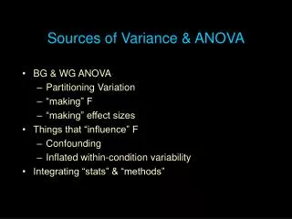
Sources of Variance & ANOVA. BG & WG ANOVA Partitioning Variation “making” F “making” effect sizes Things that “influence” F Confounding Inflated within-condition variability Integrating “stats” & “methods”. ANOVA AN alysis O f VA riance Variance means “variation”

E N D
Sources of Variance & ANOVA • BG & WG ANOVA • Partitioning Variation • “making” F • “making” effect sizes • Things that “influence” F • Confounding • Inflated within-condition variability • Integrating “stats” & “methods”
ANOVA ANalysis Of VAriance • Variance means “variation” • Sum of Squares (SS) is the most common variation index • SS stands for, “Sum of squared deviations between each of a set of values and the mean of those values” • SS = ∑ (value – mean)2 • So, Analysis Of Variance translates to “partitioning of SS” • In order to understand something about “how ANOVA works” we need to understand how BG and WG ANOVAs partition the SS differently and how F is constructed by each.
Variance partitioning for a BG design Called “error” because we can’t account for why the folks in a condition -- who were all treated the same – have different scores. Tx C 20 30 10 30 10 20 20 20 Mean 15 25 Variation among all the participants – represents variation due to “treatment effects” and “individual differences” Variation among participants within each condition – represents “individual differences” Variation between the conditions – represents variation due to “treatment effects” SSTotal=SSEffect+SSError
Constructing BG F & r SSTotal= SSEffect + SSError • Mean Square is the SS converted to a “mean” dividing it by “the number of things” • MSEffect = • MSerror = SSEffect/ dfIV dfEffect= k - 1 represents designsize SSerror / dferror dferror = ∑n – k represents sample size MSIV F is the ratio of “effect variation” (mean difference) * “individual variation” (within condition differences) F = MSerror r2 = Effect / (Effect+ error) conceptual formula = SSEffect / ( SSEffect + SSerror) definitional formula = F / (F + dferror) computational forumla
An Example … SStotal = SSeffect + SSerror 1757.574 = 605.574 + 1152.000 r2 = SSeffect / ( SSeffect + SSerror ) = 605.574 / ( 605.574 + 1152.000 ) = .34 r2 = F / (F + dferror) = 9.462 / ( 9.462 + 18) = .34
Variance partitioning for a WG design Called “error” because we can’t account for why folks who were in the same two conditions -- who were all treated the same two ways – have different difference scores. Sum Dif Tx C 20 30 10 30 10 20 20 20 50 40 30 40 10 20 10 0 Mean 15 25 Variation among participant’s difference scores – represents “individual differences” Variation among participants – estimable because “S” is a composite score (sum) SSTotal= SSEffect + SSSubj + SSError
Constructing WG F & r SSTotal= SSEffect + SSSubj+ SSError • Mean Square is the SS converted to a “mean” dividing it by “the number of things” • MSeffect= • MSerror = SSeffect / dfeffect dfeffect = k - 1 represents designsize SSerror / dferror dferror = (k-1)(s-1)represents sample size F is the ratio of “effect variation” (mean difference) * “individual variation” (within condition differences). “Subject variation” is neither effect nor error, and is left out of the F calculation. MSeffect F = MSerror r2 = effect / (effect+ error) conceptual formula = SSeffect / ( SSeffect + SSerror) definitional formula = F / (F + dferror) computational forumla
An Example … Don’t ever do this with real data !!!!!! SStotal = SSeffect + SSsubj + SSerror 1757.574 = 605.574 + 281.676 + 870.325 Professional statistician on a closed course. Do not try at home! r2 = SSeffect / ( SSeffect + SSerror ) = 605.574 / ( 605.574 + 281.676 ) = .68 r2 = F / (F + dferror) = 19.349 / ( 19.349 + 9) = .68
What happened?????Same data. Same means & Std. Same total variance. Different F ??? BG ANOVASSTotal= SSEffect + SSError WG ANOVASSTotal= SSEffect + SSSubj + SSError The variation that is called “error” for the BG ANOVA is divided between “subject” and “error” variation in the WG ANOVA. Thus, the WG F is based on a smaller error term than the BG F and so, the WG F is generally larger than the BG F. It is important to note that the dferror also changes… BG dfTotal = dfEffect + dfError WG dfTotal = dfEffect+ dfSubj + dfError So, whether F-BG or F-WG is larger depends upon how much variation is due to subject variability
What happened?????Same data. Same means & Std. Same total variance. Different r ??? r2 = Effect / (Effect+ error) conceptual formula = SSEffect / ( SSEffect + SSerror) definitional formula = F / (F + dferror) computational forumla The variation that is called “error” for the BG ANOVA is divided between “subject” and “error” variation in the WG ANOVA. Thus, the WG r is based on a smaller error term than the BG r and so, the WG r is generally larger than the BG r.
Control, variance partitioning & F… • ANOVA was designed to analyze data from studies with… • Samples that represent the target populations • True Experimental designs • proper RA • well-controlled IV manipulation • Good procedural standardization • No confounds ANOVA is a very simple statistical model that assumes there are few sources of variability in the data SSEffect / dfEffect BGSSTotal= SSEffect + SSError F = WG SSTotal= SSEffect +SSSubj+SSError SSerror / dferror However, as we’ve discussed, most data we’re asked to analyze are not from experimental designs.
2 other sources of variation we need to consider whenever we are working with quasi- or non-experiments are… • Between-condition procedural variation -- confounds • any source of between-condition differences other than the IV • subject variable confounds (initial equiv) • procedural variable confounds (ongoing equiv.) • influence the numerator of F • Within-condition procedural variation– (sorry, no agreed-upon label) • any source of within-condition differences other than “naturally occurring population individual differences” • subject variable diffs not representing the population • procedural variable influences on within cond variation • influence the denominator of F
These considerations lead us to a somewhat more realistic model of the variation in the DV… SSTotal=SSIV+SSconfound+SSindif+SSwcvar Sources of variability… SSIV IV SSconfound initial & ongoing equivalence problems SSindif population individual differences SSwcvar non-population individual differences
Imagine an educational study that compares the effects of two types of math instruction (IV)uponperformance (% - DV) Participants were randomly assigned to conditons, treated, then allowed to practice (Prac) as many problems as they wanted to before taking the DV-producing test Control GrpExper. Grp PracDV PracDV S15 75 S210 82 S35 74 S4 1084 S51078 S615 88 S71079S8 1589 • Confounding due to Practice • mean prac dif between cond • WC variability due to Practice • wg corrrelation or prac & DV • IV • compare Ss 5&2 - 7&4 • Individual differences • compare Ss 1&3, 5&7, 2&4, or 6&8
SSIV+SSconfound/ dfIV SSEffect / dfEffect F = ≠ SSindif+SSWCVAR/ dferror SSerror / dferror r = F / (F + dferror) • The problem is that the F-formula will … • Ignore the confounding caused by differential practice between the groups and attribute all BG variation to the type of instruction (IV) overestimating the SSeffect • Ignore the changes in within-condition variation caused by differential practice within the groups and attribute all WG variation to individual differences overestimating SSerror • As a result, the F & r values won’t properly reflect the relationship between type of math instruction and performance we will make statistical conclusion errors ! • We have 2 strategies: • Identify and procedurally control “inappropriate” sources • Include those sources in our statistical analyses
Both strategies require that we have a “richer” model for SS sources – and that we can apply that model to our research! The “better” SS model we’ll use … SSTotal =SSIV+ SSsubcon+ SSproccon + SSIndif+ SSwcsubinf+SSwcprocinf Sources of variability… SSIV IV SSsubcon subject variable confounds (initial eq problems) SSproccon procedural variable confounds (ongoing eq pbms) SSindif population individual differences SSwcsubinf within-condition subject variable influences SSwcprocinf within-condition procedural variable influences
Both strategies require that we have a “richer” model for variance sources – and that we can apply that model to our research! The “better” SS model we’ll use … SSTotal =SSIV+SSsubcon+ SSproccon + SSIndif+ SSwcsubinf+SSwcprocinf • In order to apply this model, we have to understand: • How these variance sources relate to aspects of … • IV manipulation & Population selection • Initial equivalence & ongoing equivalence • Sampling & procedural standardization • How these variance sources befoul SSEffect, SSerror & F of the simple ANOVA model • SSIVnumerator • SSdenominator
Sources of variability their influence on SSEffect, SSerror & F… • SSIV IV • “Bigger manipulations” produce larger mean differences • larger SSeffect larger numerator larger F • eg 0 v 50 practices instead of 0 v 25 practices • eg those receiving therapy condition get therapy twice a week instead of once a week • “Smaller manipulations” produce smaller mean differences • smaller SSeffect smaller numerator smaller F • eg 0 v 25mg antidepressant instead of 0 v 75mg • eg Big brother sessions monthly instead of each week
Sources of variability their influence on SSEffect, SSerror & F… • SSindif Individual differences • More homogeneous populations have smaller within-condition differences • smaller SSerror smaller denominator larger F • eg studying one gender instead of both • eg studying “4th graders” instead of “grade schoolers” • More heterogeneous populations have larger within-condition differences • larger SSerror larger denominator smaller F • eg studying “young adults” instead of “college students” • eg studying “self-reported” instead of “vetted” groups
Sources of variability their influence on SSEffect, SSerror & F… • The influence a confound has on SSIV & F depends upon the “direction of the confounding” relative to “the direction of the IV” • if the confound “augments” the IV SSIV & F will be inflated • if the confound “offsets” the IV SSIV & F will be deflated • SSsubcon subject variable confounds (initial eq problems) • Augmenting confounds • inflates SSEffect inflates numerator inflates F • eg 4th graders in Tx group & 2nd graders is Cx group • eg run Tx early in semester and Cx at end of semester • Offsetting confounds • deflates SSEffect deflates denominator deflates F • eg 2nd graders in Tx group & 4th graders is Cx group • eg “better neighborhoods” in Cx than in Tx
Sources of variability their influence on SSEffect, SSerror & F… • The influence a confound has on SSIV & F depends upon the “direction of the confounding” relative to “the direction of the IV” • if the confound “augments” the IV SSIV & F will be inflated • if the confound “offsets” the IV SSIV & F will be deflated • SSproccon procedural variable confounds (ongoing eq problems) • Augmenting confounds • inflates SSEffect inflates numerator inflates F • eg Tx condition is more interesting/fun for assistants to run • eg Run the Tx on the newer, nicer equipment • Offsetting confounds • deflates SSEffect deflates denominator deflates F • eg less effort put into instructions for Cx than for Tx • eg extra practice for touch condition than for visual cond
Sources of variability their influence on SSEffect, SSerror & F… • The influence this has on SSError & F depends upon the whether the sample is more or less variable than the target pop • if “more variable” SSError is inflated & F will be deflated • if “less variable” SSError is deflated & F will be inflated • SSwcsubinf within-condition subjectvariable influences • More variation in the sample than in the population • inflates SSError inflates denominator deflates F • eg target pop is “3rd graders” - sample is 2nd 3rd & 4th graders • eg target pop is “clinically anxious” – sample is “anxious” • Less variation in the sample than in the population • deflates SSError deflates denominator inflates F • eg target pop is “grade schoolers” – sample is 4th graders • eg target pop is “young adults” – sample is college students
Sources of variability their influence on SSEffect, SSerror & F… • The influence this has on SSError & F depends upon the whether the procedure leads to more or less within condition variance in the sample data than would be in the population • if “more variable” SSError is inflated & F will be deflated • if “less variable” SSError is deflated & F will be inflated • SSwcsubinf within-condition procedural variable influences • More variation in the sample data than in the population • inflates SSError inflates denominator deflates F • eg letting participants practice as much as they want • eg using multiple research stations • Less variation in the sample data than in the population • deflates SSError deflates denominator inflates F • eg DV measures that have floor or ceiling effects • eg time allotments that produce floor or ceiling effects
Couple of important things to note !!! SSTotal =SSIV+SSsubcon+ SSproccon + SSIndif+ SSwcsubinf+SSwcprocinf • Most variables that are confounds also inflate within condition variation!!! • like in the simple example earlier • “Participants were randomly assigned to conditons, treated, then allowed to practice as many problems as they wanted to before taking the DV-producing test”
Couple of important things to note !!! SSTotal =SSIV+SSsubcon+ SSproccon + SSIndif+ SSwcsubinf+SSwcprocinf • There is an important difference between “picking a population that has more/less variation” and “sampling poorly so that your sample has more/less variation than the population”. • is you intend to study 3rd, 4th & 5th graders instead of just 3rd graders, your SSerror will increase because your SSindif will be larger – but it is a choice, not a mistake!!! • if intend to study 3rd stage cancer patients, but can’t find enough and use 2nd, 3rd & 4th stage patients instead, your SSerror will be inflated because of your SSwcsubinf – and that is a mistake not a choice!!!