Download
1 / 39
390 likes | 505 Views
Assimilating Earth Observation Data into VEGETATION MODELS. Tristan Quaife DARC seminar 11 th July 2012. Some context – the residual sink. PgCyr -1. http://www.whrc.org/global/carbon/residual.html. Some context – Cox et al. 2000. Change in vegetation carbon (GtC). 0. 0.

E N D
Assimilating Earth Observation Data into VEGETATION MODELS Tristan Quaife DARC seminar 11th July 2012
Some context – the residual sink PgCyr-1 http://www.whrc.org/global/carbon/residual.html
Some context – Cox et al. 2000 Change in vegetation carbon (GtC) 0 0 The red lines represent the fully coupled climate/carbon-cycle simulation, and the blue lines are from the 'offline' simulation which neglects direct CO2-induced climate change. The figure shows simulated changes in vegetation carbon (a) and soil carbon (b) for the global land area (continuous lines) and South America alone (dashed lines). Cox P et al. (2000) Acceleration of global warming due to carbon-cycle feedbacks in a coupled climate model. Nature. 408, 184-187
The Land Surface DA problem • At first glance similar to NWP DA problem. Of the form: xt+1=M(xt, p, dt) • But… • Observation time scales tend to be much shorter than many of the key process • In general M is not fully understood and typical for many parameters to be determined empirically
Assimilating products Assumptions Observations Data Assimilation Scheme (KF, EnKF, 4DVAR, etc) Assumptions Observations MODEL Assumptions For example: soil moisture from SMOS or photosynthesis (GPP) from MODIS
MODIS GPP/PSN MODIS data Look up table Climate data http://www.ntsg.umt.edu/remote_sensing/netprimary/
Observation Operator MODEL Assumptions Assumptions Assimilating low level data Data Assimilation Scheme (KF, EnKF, 4DVAR, etc) Observations Observations e.g. reflectance, backscatter, etc… Quaife T, Lewis P, De Kauwe M, Williams M, Law BE, Disney MI and Bowyer P (2008) Assimilating canopy reflectance data into an ecosystem model with an Ensemble Kalman Filter. Remote Sensing of Environment. 112(4):1347-1364
Af Lf Foliage Rh Ra Lr Ar GPP Roots Litter D Met Data Lw Aw Wood Humus Vegetation Soil DALEC
Ensemble Kalman Filter Aa = A + A′A′THT(HA′A′THT + Re)-1(D - HA) H = observation operator A = state vector ensemble A′ = state vector ensemble – mean state vector D = observation ensemble Re= observation error covariance matrix
EnKF – augmented analysis Aa = A + A′Â′TĤT(ĤÂ′Â′TĤT + Re)-1(D - ĤÂ) Ĥ= augmented observation operator Â= augmentedstate vector ensemble Â= h(A) A h is a canopy reflectance model
Observation operator Source: N Gobron, JRC
Geometric Observation Operator Shaded crown Illuminated crown Illuminated soil Shaded soil
Modelled vs. observed reflectance MODIS Band 1 (red) MODIS Band 2 (NIR) Quaife T, Lewis P, De Kauwe M, Williams M, Law BE, Disney MI and Bowyer P (2008) Assimilating canopy reflectance data into an ecosystem model with an Ensemble Kalman Filter. Remote Sensing of Environment. 112(4):1347-1364
Assimilating reflectance into DALEC No assimilation Assimilating MODIS surface reflectance bands 1 and 2
15 65 gC/m2/year Carbon balance for 2000-2002 Flux Tower 4.5 km Spatial average = 50.9 Std. dev. = 9.7 (gC/m2/year)
Parameter sensitivity • Problem using optical EO data is most vegetation model parameters are not sensitive to it • Broadly this is true for all EO data • May change with advent of CO2 observations • Have taken a different approach for some problems: • Use models driven by satellite data • Assimilate available ground data
Mountain pine beetles • Science question: what is the impact of MPB on carbon balance of ecosystem? • Problem: most veg models are not adequately parameterised for mountain forests • tend to exhibit quite different photosynthetic responses to temperature than other forests • Use simple photosynthesis model driven by EO data • Assimilate ground observations using standard MCMC-MH Bayesian parameter estimation
Mountain pine beetle Moore DJP, Trahan NA, Wilkes P, Quaife T, Desai AR, Negron JF, Stephens BB, Elder K & Monson RK (submitted 2012) Changes in carbon balance after insect disturbance in Western U.S. Forests.
A re-think… • Started to think about how we could approach the land surface problem a little differently • First, most land surface models do not have RT physics that is consistent with EO observations • Make this a design goal of vegetation models • A good place to start given volume of EO data • Second, there may be additional constraints that are applicable specifically to the land surface • Generally does not undergo rapid change
Kernel driven BRDF model λ = wavelength ρ = BRF Ω = view geometry Ω' = illumination geometry f = kernel weight K = kernel value n = number of kernels
Standard Least Squares f = (KTC-1K)-1KTC-1ρ • Formulation used for the NASA MODIS BRDF/albedo product (MCD43) • Requires an 16 day window (Terra + Aqua) that is moved every 8 days
Constrained formulation f = (KTC-1K + γ2BTB)-1KTC-1ρ B is the required constraint. It imposes: Bf = 0 and the scalar γ is a weighting on that constraint.
Constrained result Quaife T and Lewis P (2010) Temporal Constraints on Linear BRDF Model Parameters. IEEE Transactions on Geoscience and Remote Sensing, 48 (5). pp. 2445-2450.
EOLDAS • European Space Agency Project to improve data retrievals and inter-sensor calibration • Variational scheme using the following cost function:
EOLDAS variational assimilation Leaf Area Index Chlorophyll Time Lewis P, Gomez-Dans J, Kaminski T, Settle J, Quaife T, Gobron N, Styles J & Berger M (2012), An Earth Observation Land Data Assimilation System (EOLDAS), Remote Sensing of Environment.
Spatial DA example – Synthetic Truth NDVI Source: P Lewis & J Gomez-Dans, UCL
Spatial DA example – Observations NDVI Source: P Lewis & J Gomez-Dans, UCL
Spatial DA example – Posterior NDVI Source: P Lewis & J Gomez-Dans, UCL
Multi-scale DA using a particle filter Leaf Area Index: Hill TC, Quaife T & Williams M (2011) A data assimilation method for using low-resolution Earth observation data in heterogeneous ecosystems, J. Geophys. Res., 116, D08117.
Current ESA project • Project with Reading and UCL • Builds on the existing EOLDAS framework • Constructing a land surface scheme that includes trace gas and energy fluxes • Key aim is to have the broadest possible range of EO observations available for DA • Design goal to invest most complexity in the physics required for the observation operator
Routes to collaboration inside DARC • DALEC code setup in flexible framework • Already has EnKF& PF – easy to add more • Easy to add non-linear observation operators • Lots of test data available • EOLDAS code available • Official public release very soon • Very general, but also very slow • Lots of data for vegetation type problems available… ask me…