Chapter 3: Model Testing and Selection

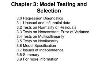
1. Chapter 3: Model Testing and Selection     3.0 Regression Diagnostics    3.1 Unusual and Influential data    3.2 Tests on Normality of Residuals    3.3 Tests on Nonconstant Error of Variance    3.4 Tests on Multicollinearity    3.5 Tests on Nonlinearity    3.6 Model Specification    3.7 Issues of Independence    3.8 Summary    3.9 For more information

2. Regression Examine In last chapter, we learned how to do for regression with SAS. This chapter show how readers can use SAS to test whether data meet the assumptions of linear regression.  Linearity - the relationships between the predictors and the outcome variable should be linear Normality - the errors should be normally distributed - technically normality is necessary only for the t-tests, estimation of the coefficients only requires that the errors be iid Homogeneity of variance: the error variance should be constant Independence - the errors associated with one observation are not correlated with the errors of any other observation No errors in pred variables - predictor variables are measured without error Model specification - the model should be properly specified (including all relevant variables, and excluding irrelevant variables) Influence - individual observations (such as outliers) that exert undue influence on the coefficients Collinearity - predictors that are highly collinear, i.e. linearly related, can cause problems in estimating the regression coefficients

3. 3.1 Unusual and Influential data A single observation that is substantially different from all other observations can make a large difference in the results of regression analysis.  If a single observation (or small group of observations) substantially changes results, we should know about this and investigate further.  There are three ways that an observation can be unusual. Outliers: an outlier is an observation with large residual. In other words, it is an observation whose dependent-variable value is unusual given its values on the predictor variables. An outlier may indicate a sample peculiarity or may indicate a data entry error or other problem. Leverage: An observation with an extreme value on a predictor variable is called a point with high leverage. Leverage is a measure of how far an independent variable deviates from its mean. These leverage points can have an effect on the estimate of regression coefficients. (In multi-linear regression, high leverage points are those that are outliers with respect to the independent variables. Influential points are those that cause large changes in the parameter estimates when they are deleted. Although an influential point will typically have high leverage, a high leverage point is not necessarily an influential point. The leverage is typically defined as the diagonal of the hat matrix (hat matrix H = X(X'X)-1X'). Influence: An observation is said to be influential if removing the observation substantially changes the estimate of coefficients. Influence can be thought of as the product of leverage and outlierness.

4. Leverage The “hat value” measures the leverage of a particular case. For simple regression (i.e., 1 independent variable), this measures the difference of from the mean of X. And in multiple regression, it is a measure of how far case i is from the mean of all the independent variables in the model.

5. studentized residual Run the regression excluding case j. Then predict the value of case j using the coefficients from this regression. The studentized residual is

6. DFBETA and Cook’s D DFBETA is the impact on each coefficient deleting each observation in turn, for all coefficients j and cases I Dij=Bj-bj(-i) Cook’s D is the standardized residual times leverage = a measure of influence

7. Parital-regression plots (= added-variable plots) Visual depiction of influential cases: Three steps for an av-plot of Y on X1: 1) regress Y on the independent variables, excluding X1. Calculate the residuals. 2) regress X1 on the other ind. variables. Calculate the residuals. 3) graph the residuals from #1 by the residuals from #2 ---this allows you to look at the relationship between Y and X1, taking out the effect of the other variables.

8. Examine the data proc contents data="c:\sasreg\crime"; run; The CONTENTS Procedure Data Set Name: c:\sasreg\crime Observations: 51 Member Type: DATA Variables: 9 Engine: V8 Indexes: 0 Created: 4:58 Saturday, January 9, 1960 Observation Length: 63 Last Modified: 4:58 Saturday, January 9, 1960 Deleted Observations: 0 Protection: Compressed: NO Data Set Type: Sorted: NO Label: < some output omitted to save space> -----Alphabetic List of Variables and Attributes----- # Variable Type Len Pos Label --------------------------------------------------------- 3 crime Num 4 8 violent crime rate 4 murder Num 8 12 murder rate 7 pcths Num 8 36 pct hs graduates 5 pctmetro Num 8 20 pct metropolitan 6 pctwhite Num 8 28 pct white 8 poverty Num 8 44 pct poverty 1 sid Num 8 0 /*state id*/ 9 single Num 8 52 pct single parent 2 state Char 3 60 /*state name*/

9. Examine the mean value proc means data="c:\sasreg\crime"; var crime murder pctmetro pctwhite pcths poverty single; run; The MEANS Procedure Variable Label N Mean Std Dev Minimum ------------------------------------------------------------------------------- crime violent crime rate 51 612.8431373 441.1003229 82.0000000 murder murder rate 51 8.7274510 10.7175758 1.6000000 pctmetro pct metropolitan 51 67.3901959 21.9571331 24.0000000 pctwhite pct white 51 84.1156860 13.2583917 31.7999992 pcths pct hs graduates 51 76.2235293 5.5920866 64.3000031 poverty pct poverty 51 14.2588235 4.5842416 8.0000000 single pct single parent 51 11.3254902 2.1214942 8.3999996 ------------------------------------------------------------------------------- Variable Label Maximum -------------------------------------------- crime violent crime rate 2922.00 murder murder rate 78.5000000 pctmetro pct metropolitan 100.0000000 pctwhite pct white 98.5000000 pcths pct hs graduates 86.5999985 poverty pct poverty 26.3999996 single pct single parent 22.1000004 --------------------------------------------

10. Observation • Suppose to predict crime by pctmetro, poverty, and single by building a linear regression model between the response variable crime and the independent variables pctmetro, poverty and single. • First look at the scatter plots of crime against each of the predictor variables before the regression analysis so we will have some ideas about potential problems. We can create a scatterplot matrix of these variables as shown below.

11. Checking by Graph proc insight data="c:\sasreg\crime"; scatter crime pctmetro poverty single* crime pctmetro poverty single; run; quit; The graphs of crime with other variables in the next chart show some potential problems.  In every plot, we see a data point that is far away from the rest of the data points. Let's make individual graphs of crime with pctmetro and poverty and single so we can get a better view of these scatterplots.  We will add the pointlabel = ("#state") option in the symbol statement to plot the state name instead of a point.

13. Check (continuous) goptions reset=all; axis1 label=(r=0 a=90); symbol1 pointlabel = ("#state") font=simplex value=none; 1. proc gplot data="c:\sasreg\crime"; plot crime*pctmetro=1 / vaxis=axis1; run; quit; 2. proc gplot data="c:\sasreg\crime"; plot crime*poverty=1 / vaxis=axis1; run; quit; 3. proc gplot data="c:\sasreg\crime"; plot crime*single=1 / vaxis=axis1; run; quit;

17. Discussion All the scatter plots suggest that the observation for state = dc is a point that requires extra attention since it stands out away from all of the other points. We will keep it in mind when we do our regression analysis. Now let's try the regression command predicting crime from pctmetro,poverty and single.  We will go step-by-step to identify all the potentially unusual or influential points afterwards. We will output several statistics that we will need for the next few analyses to a dataset called crime1res, and we will explain each statistic in turn.  These statistics include the studentized residual (called r), leverage (called lev), Cook's D (called cd) and DFFITS (called dffit).  We are requesting all of these statistics now so that they can be placed in a single dataset that we will use for the next several examples.  Otherwise, we could have to rerun the proc reg each time we wanted a new statistic and save that statistic to another output data file.

18. Regression Program proc reg data="c:\sasreg\crime"; model crime=pctmetro poverty single; output out=crime1res(keep=sid state crime pctmetro poverty single r lev cd dffit) rstudent=r h=lev cookd=cd dffits=dffit; run; quit;

19. Output The REG Procedure Model: MODEL1 Dependent Variable: crime violent crime rate Analysis of Variance Sum of Mean Source DF Squares Square F Value Pr > F Model 3 8170480 2723493 82.16 <.0001 Error 47 1557995 33149 Corrected Total 50 9728475 Root MSE 182.06817 R-Square 0.8399 Dependent Mean 612.84314 Adj R-Sq 0.8296 Coeff Var 29.70877 Parameter Estimates Parameter Standard Variable Label DF Estimate Error t Value Pr > |t| Intercept Intercept 1 -1666.43589 147.85195 -11.27 <.0001 pctmetro pct metropolitan 1 7.82893 1.25470 6.24 <.0001 poverty pct poverty 1 17.68024 6.94093 2.55 0.0142 single pct single parent 1 132.40805 15.50322 8.54 <.0001

20. Examine Residuals Let's examine the studentized residuals as a first means for identifying outliers. We requested the studentized residuals in the above regression in the output statement and named them r. We can choose any name we like as long as it is a legal SAS variable name. Studentized residuals are a type of standardized residual that can be used to identify outliers. Let's examine the residuals with a stem and leaf plot. We see three residuals that stick out, -3.57, 2.62 and 3.77.  proc univariate data=crime1res plots plotsize=30; var r; run;

21. The UNIVARIATE Procedure Variable: r (Studentized Residual without Current Obs) Moments N 51 Sum Weights 51 Mean 0.0184024 Sum Observations 0.93852247 Std Deviation 1.1331258 Variance 1.28397408 Skewness 0.2243412 Kurtosis 3.05611851 Uncorrected SS 64.215975 Corrected SS 64.198704 Coeff Variation 6157.48877 Std Error Mean 0.15866935 Basic Statistical Measures Location Variability Mean 0.018402 Std Deviation 1.13313 Median 0.052616 Variance 1.28397 Mode . Range 7.33664 Interquartile Range 1.19867 Tests for Location: Mu0=0 Test -Statistic- -----p Value------ Student's t t 0.11598 Pr > |t| 0.9081 Sign M 0.5 Pr >= |M| 1.0000 Signed Rank S -1 Pr >= |S| 0.9926

22. Quantile Estimate 100% Max 3.7658467 99% 3.7658467 95% 1.5896441 90% 1.0767182 75% Q3 0.6374511 50% Median 0.0526162 25% Q1 -0.5612179 10% -1.1293398 5% -1.6855980 1% -3.5707892 0% Min -3.5707892 Extreme Observations ------Lowest----- -----Highest----- Value Obs Value Obs -3.57079 25 1.15170 14 -1.83858 18 1.29348 13 -1.68560 39 1.58964 12 -1.30392 47 2.61952 9 -1.14833 35 3.76585 51

23. Stem Leaf # Boxplot 3 8 1 0 3 2 6 1 0 2 1 6 1 | 1 000123 6 | 0 5566788 7 +-----+ 0 1111333344 10 *--+--* -0 4433210 7 | | -0 9976655555 10 +-----+ -1 31100 5 | -1 87 2 | -2 -2 -3 -3 6 1 0 ----+----+----+----+

24. Normal Probability Plot 3.75+ * | | * ++++ 2.25+ ++++ | ++*+ | +**** * 0.75+ +**** | ******* | ****** -0.75+ *****+ | * ****+ | * +*++ -2.25+ +++++ |+++ | -3.75+ * +----+----+----+----+----+----+----+----+----+----+ -2 -1 0 +1 +2

25. The stem and leaf display helps us see some potential outliers, but we cannot see which state (which observations) are potential outliers.  Let's sort the data on the residuals and show the 10 largest and 10 smallest residuals along with the state id and state name.   proc sort data=crime1res; by r; run; proc print data=crime1res(obs=10); run; Obs sid state r 1 25 ms -3.57079 2 18 la -1.83858 3 39 ri -1.68560 4 47 wa -1.30392 5 35 oh -1.14833 6 48 wi -1.12934 7 6 co -1.04495 8 22 mi -1.02273 9 4 az -0.86992 10 44 ut -0.85205 proc print data=crime1res(firstobs=42 obs=51); var sid state r; run; Obs sid state r 42 24 mo 0.82117 43 20 md 1.01299 44 29 ne 1.02887 45 40 sc 1.03034 46 16 ks 1.07672 47 14 il 1.15170 48 13 id 1.29348 49 12 ia 1.58964 50 9 fl 2.61952 51 51 dc 3.76585

26. Outliers identification We should pay attention to studentized residuals that exceed +2 or -2, and get even more concerned about residuals that exceed +2.5 or -2.5 and even yet more concerned about residuals that exceed +3 or -3.  These results show that DC and MS are the most worrisome observations, followed by FL. Let's show all of the variables in our regression where the studentized residual exceeds +2 or -2, i.e., where the absolute value of the residual exceeds 2.  We see the data for the three potential outliers we identified, namely Florida, Mississippi and Washington D.C. Looking carefully at these three observations, we couldn't find any data entry errors, though we may want to do another regression analysis with the extreme point such as DC deleted. We will return to this issue later.  

27. Print outliers proc print data=crime1res; var r crime pctmetro poverty single; where abs(r)>2; run; Obs r crime pctmetro poverty single 1 -3.57079 434 30.700 24.7000 14.7000 50 2.61952 1206 93.000 17.8000 10.6000 51 3.76585 2922 100.000 26.4000 22.1000

28. Identify leverage Now let's look at the leverage's to identify observations that will have potential great influence on regression coefficient estimates.   proc univariate data=crime1res plots plotsize=30; var lev; run; The UNIVARIATE Procedure Variable: lev (Leverage) Moments N 51 Sum Weights 51 Mean 0.07843137 Sum Observations 4 Std Deviation 0.0802847 Variance 0.00644563 Skewness 4.16424136 Kurtosis 21.514892 Uncorrected SS 0.63600716 Corrected SS 0.32228167 Coeff Variation 102.362995 Std Error Mean 0.01124211 Basic Statistical Measures Location Variability Mean 0.078431 Std Deviation 0.08028 Median 0.061847 Variance 0.00645 Mode . Range 0.51632 Interquartile Range 0.04766 Tests for Location: Mu0=0 Test -Statistic- -----p Value------ Student's t t 6.976572 Pr > |t| <.0001 Sign M 25.5 Pr >= |M| <.0001 Signed Rank S 663 Pr >= |S| <.0001

29. Quintiles Quantile Estimate 100% Max 0.5363830 99% 0.5363830 95% 0.1910120 90% 0.1362576 75% Q3 0.0851089 50% Median 0.0618474 25% Q1 0.0374442 10% 0.0292452 5% 0.0242659 1% 0.0200613 0% Min 0.0200613 Extreme Observations -------Lowest------ ------Highest----- Value Obs Value Obs 0.0200613 38 0.165277 2 0.0241210 6 0.180201 15 0.0242659 22 0.191012 1 0.0276638 17 0.260676 32 0.0287552 5 0.536383 51

30. Stem Leaf Plot Stem Leaf # Boxplot 52 6 1 * 50 48 46 44 42 40 38 36 34 32 30 28 26 1 1 * 24 22 20 18 01 2 0 16 5 1 0 14 12 6 1 | 10 02 2 | 8 2355515 7 +-----+ 6 0123344722366 13 *--+--* 4 35567907 8 | | 2 044899112245789 15 +-----+ ----+----+----+----+

31. Norm-ability Plot Normal Probability Plot 0.53+ * | | | | 0.43+ | | | | 0.33+ | | | * +++ | ++ 0.23+ +++ | ++ | ++** | ++* | +++ 0.13+ ++ * | +++ * | ++ ***** | +******* | ***** 0.03+ * * ** ********+ +----+----+----+----+----+----+----+----+----+----+ -2 -1 0 +1 +2 

32. Extreme value of leverage proc sort data=crime1res; by lev; run; proc print data=crime1res (firstobs=42 obs=51); var lev state; run; Obs lev state 42 0.09114 ky 43 0.09478 nj 44 0.09983 mt 45 0.10220 fl 46 0.13626 vt 47 0.16528 la 48 0.18020 wv 49 0.19101 ms 50 0.26068 ak 51 0.53638 dc

33. Leverage Evaluation Generally, a point with leverage greater than (2k+2)/n should be carefully examined, where k is the number of predictors and n is the number of observations. In our example this works out to (2*3+2)/51 = .15686275, so we can do the following. proc print data=crime1res; var crime pctmetro poverty single state; where lev > .156; run; Obs crime pctmetro poverty single state 47 1062 75.000 26.4000 14.9000 la 48 208 41.800 22.2000 9.4000 wv 49 434 30.700 24.7000 14.7000 ms 50 761 41.800 9.1000 14.3000 ak 51 2922 100.000 26.4000 22.1000 dc

34. Further Examine DC is an observation that both has a large residual and large leverage.  Such points are potentially the most influential.  We can make a plot that shows the leverage by the residual squared and look for observations that are jointly high on both of these measures.  We can do this using a leverage versus residual-squared plot. Using residual squared instead of residual itself, the graph is restricted to the first quadrant and the relative positions of data points are preserved. This is a quick way of checking potential influential observations and outliers at the same time. Both types of points are of great concern for us.  

35. proc sql; create table crimeres5 as select *, r**2/sum(r) as rsquared from crime1res; quit; goptions reset=all; axis1 label=(r=0 a=90); symbol1 pointlabel = ("#state") font=simplex value=none; proc gplot data=crimeres5; plot lev*rsquared / vaxis=axis1; run; quit;

37. The point for DC catches our attention having both the highest residual squared and highest leverage, suggesting it could be very influential. The point for MS has almost as large a residual squared, but does not have the same leverage.  We'll look at those observations more carefully by listing them below. proc print data="c:\sasreg\crime"; where state="dc" or state="ms"; var state crime pctmetro poverty single; run; Obs state crime pctmetro poverty single 25 ms 434 30.700 24.7000 14.7000 51 dc 2922 100.000 26.4000 22.1000

38. Cook's D and DFITS Now let's move on to overall measures of influence. Specifically, let's look at Cook's D and DFITS.  These measures both combine information on the residual and leverage. Cook's D and DFITS are very similar except that they scale differently, but they give us similar answers. The lowest value that Cook's D can assume is zero, and the higher the Cook's D is, the more influential the point is. The conventional cut-off point is 4/n. We can list any observation above the cut-off point by doing the following. We do see that the Cook's D for DC is by far the largest. 

39. Cook’sD proc print data=crime1res; where cd > (4/51); var crime pctmetro poverty single state cd; run; Obs crime pctmetro poverty single state cd 45 1206 93.000 17.8000 10.6000 fl 0.17363 47 1062 75.000 26.4000 14.9000 la 0.15926 49 434 30.700 24.7000 14.7000 ms 0.60211 51 2922 100.000 26.4000 22.1000 dc 3.20343

40. DFITS Now let's take a look at DFITS. The conventional cut-off point for DFITS is 2*sqrt(k/n). DFITS can be either positive or negative, with numbers close to zero corresponding to the points with small or zero influence. As we see, DFITS also indicates that DC is, by far, the most influential observation. proc print data=crime1res; where abs(dffit)> (2*sqrt(3/51)); var crime pctmetro poverty single state dffit; run; Obs crime pctmetro poverty single state dffit 45 1206 93.000 17.8000 10.6000 fl 0.88382 47 1062 75.000 26.4000 14.9000 la -0.81812 49 434 30.700 24.7000 14.7000 ms -1.73510 51 2922 100.000 26.4000 22.1000 dc 4.05061

41. DFBETA • The above measures are general measures of influence.  Readers can also consider more specific measures of influence that assess how each coefficient is changed by deleting the observation. This measure is called DFBETA and is created for each of the predictors. Apparently this is more computationally intensive than summary statistics such as Cook's D because the more predictors a model has, the more computation it may involve. We can restrict our attention to only those predictors that we are most concerned with and  to see how well behaved those predictors are. In SAS, we need to use the ods output OutStatistics statement to produce the DFBETAs for each of the predictors. The names for the new variables created are chosen by SAS automatically and begin with DFB_. 

42. SAS Progrqm for dfbeta proc reg data="c:\sasreg\crime"; model crime=pctmetro poverty single / influence; ods output OutputStatistics=crimedfbetas; id state; run; proc print data=crimedfbetas (obs=5); var state DFB_pctmetro DFB_poverty DFB_single; run;

43. RESULTS DFB_ DFB_ DFB_ Obs state pctmetro poverty single 1 ak -0.1062 -0.1313 0.1452 2 al 0.0124 0.0553 -0.0275 3 ar -0.0687 0.1753 -0.1053 4 az -0.0948 -0.0309 0.0012 5 ca 0.0126 0.0088 -0.0036 The value for DFB_single for Alaska is 0.14, which means that by being included in the analysis (as compared to being excluded), Alaska increases the coefficient for single by 0.14 standard errors, i.e., 0.14 times the standard error for BSingle or by (0.14 * 15.5).  Because the inclusion of an observation could either contribute to an increase or decrease in a regression coefficient, DFBETAs can be either positive or negative.  A DFBETA value in excess of  2/sqrt(n) merits further investigation. In this example, we would be concerned about absolute values in excess of 2/sqrt(51) or 0.28.

44. Plot of Dfbeta and Residual We can plot all three DFBETA values against the state id in one graph shown below. We add a line at 0.28 and -0.28 to help us see potentially troublesome observations.  We see the largest value is about 3.0 for DFsingle. data crimedfbetas1; set crimedfbetas; rename HatDiagonal=lev; run; proc sort data=crimedfbetas1; by lev; proc sort data=crime1res; by lev; run; data crimedfbetas2; merge crime1res crimedfbetas1; by lev; run; goptions reset=all; symbol1 v=circle c=red; symbol2 v=plus c=green; symbol3 v=star c=blue; axis1 order=(1 51); axis2 order=(-1 to 3.5 by .5); proc gplot data=crimedfbetas2; plot DFB_pctmetro*sid=1 DFB_poverty*sid=2 DFB_single*sid=3 / overlay haxis=axis1 vaxis=axis2 vref=-.28 .28; run; quit;

46. Plot all three goptions reset=all; axis1 label=(r=0 a=90); symbol1 pointlabel = ("#state") font=simplex value=none; proc gplot data=crimedfbetas2; plot DFB_pctmetro*sid=1 DFB_poverty*sid=2 DFB_single*sid=3 / overlay vaxis=axis1 vref=-.28 .28; run; quit;

48. DFB_single Now let's list those observations with DFB_single larger than the cut-off value.  Again, we see that DC is the most problematic observation. proc print data=crimedfbetas2; where abs(DFB_single) > 2/sqrt(51); var DFB_single state crime pctmetro poverty single; run; DFB_ Obs single state crime pctmetro poverty single 45 -0.5606 fl 1206 93.000 17.8000 10.6000 49 -0.5680 ms 434 30.700 24.7000 14.7000 51 3.1391 dc 2922 100.000 26.4000 22.1000

49. Measure of Threshold for Identifying Abnormal Observations

50. Analyses with and without DC 1. proc reg data="c:\sasreg\crime"; model crime=pctmetro poverty single; run; quit; 2. proc reg data="c:\sasreg\crime"; model crime=pctmetro poverty single; where state ne "dc"; run; quit;