Download
1 / 20
200 likes | 393 Views
Adjusting for extraneous factors. Topics for today More on logistic regression analysis for binary data and how it relates to the Wolf and Mantel-Haenszel estimates of a common odds ratios Interpreting logistic regression analysis

E N D
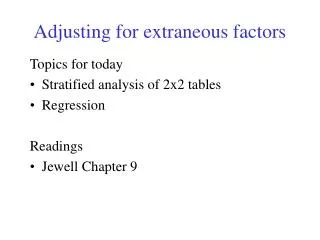
Adjusting for extraneous factors Topics for today • More on logistic regression analysis for binary data and how it relates to the Wolf and Mantel-Haenszel estimates of a common odds ratios • Interpreting logistic regression analysis • Estimating a common risk ratio in the presence of a stratification factor. Connection to Poisson regression. Readings • Jewell Chapter 9
Stratified analysis for binary data Data from the ith stratum: Variance formulae in JewellChapter 9
Regression-based stratified analysis for Berkeley data data berkeley; input stratum male a b ; cards; 1 1 512 313 1 0 89 19 2 1 353 207 2 0 17 8 3 1 120 205 3 0 202 391 4 1 138 279 4 0 131 244 5 1 53 138 5 0 94 299 6 1 22 351 6 0 24 317 run; data berkeley; set berkeley; n=a+b; procgenmod; class stratum; model a/n=male stratum/dist=binomial; run;
Stratified analysis Standard 95% Conf Chi- Parameter DF Estimate Error Limits Square Pr > ChiSq Intercept 1 -2.6246 0.1577 -2.9337 -2.3154 276.88 <.0001 male 1 -0.0999 0.0808 -0.2583 0.0586 1.53 0.2167 stratum 1 1 3.3065 0.1700 2.9733 3.6396 378.38 <.0001 stratum 2 1 3.2631 0.1788 2.9127 3.6135 333.12 <.0001 stratum 3 1 2.0439 0.1679 1.7149 2.3729 148.24 <.0001 stratum 4 1 2.0119 0.1699 1.6788 2.3449 140.18 <.0001 stratum 5 1 1.5672 0.1804 1.2135 1.9208 75.44 <.0001 stratum 6 0 0.0000 0.0000 0.0000 0.0000 . . Scale 0 1.0000 0.0000 1.0000 1.0000 Wolf estimate: -0.0746 SE= 0.0822 CI: (-0.2357, 0.0866) Mantel-Haenszel (have to take logs of this estimate): -0.1002 CI: (-0.2931, 0.0615) Lets talk about the rest of these regression results … what do they mean?
Interpreting the logistic regression model for the Berkeley data We are fitting the following model: Based on the fitted model, we can predict the admission probabilities in each cell
More on the Berkeley logistic regression analysis In addition to providing an estimate of the overall gender effect, the logistic regression analysis allows us to compare admission rates between the departments. Based on the observed data, what is the log odds ratio for admission to department 5 versus department 6 for females? What about for males? What about department 1 versus department 6 for males? Females?
Another example We can add additional factors into the logistic regression model so as to obtain an estimate of the log-odds ratio, adjusting for these additional factors. Example, smoking in the Epilepsy study. Lets look in SAS: procfreq ; table one3*cig2 /chisq; run;
Standard Wald 95% Confidence Chi- Parameter DF Estimate Error Limits Square Pr > ChiSq Intercept 1 -3.1396 0.2229 -3.5765 -2.7028 198.41 <.0001 DRUG 1 1 1.0384 0.2876 0.4748 1.6020 13.04 0.0003 DRUG 2 1 -0.2944 0.6275 -1.5243 0.9355 0.22 0.6390 DRUG 3 0 0.0000 0.0000 0.0000 0.0000 . . Scale 0 1.0000 0.0000 1.0000 1.0000 Standard Wald 95% Confidence Chi- Parameter DF Estimate Error Limits Square Pr > ChiSq Intercept 1 -3.3872 0.2435 -3.8644 -2.9100 193.55 <.0001 DRUG 1 1 1.0712 0.2939 0.4952 1.6472 13.29 0.0003 DRUG 2 1 -0.3596 0.6337 -1.6016 0.8824 0.32 0.5704 DRUG 3 0 0.0000 0.0000 0.0000 0.0000 . . CIG2 1 1.0721 0.3131 0.4585 1.6857 11.73 0.0006 Scale 0 1.0000 0.0000 1.0000 1.0000
Why don’t drug estimates change much?? Hint – look at association between drug and smoking procfreq ; table one3*cig2 /chisq; run;
Relative Risks We’ve talked about estimating odds ratios while adjusting for another factor. Several approaches: • Cochran-Mantel-Haenszel test • Wolf estimate of the adjusted logodds ratio • Mantel-Haenszel estimate of adjusted odds ratio • Logistic regression Lets turn now to analogous consideration for risk ratios or relative risks
Example from Jewell Table 9.2 Relationship between behavior (type A vs type B personality) and coronary heart disease events (see p82 in Jewell for description). Unadjusted RR was 2.2 with 95% CI of (1.72, 2.87). Since weight is important, we need to adjust for it too
CHD example Jewell table 9.7 provides the weights for the Wolf and Mantel-Haenszel methods Lets look at using Poisson regression to do the adjustment.
Fitting the CHD model in SAS data chd; input weight behavior a b; cards; 1 1 22 253 1 0 10 305 2 1 21 235 2 0 10 270 3 1 29 297 3 0 21 297 4 1 47 248 4 0 19 253 5 1 59 378 5 0 19 361 Run; data cdh; set chd; lnn=log(a+b); procgenmod; model a=behavior/dist=poisson offset=lnn; procgenmod; class weight; model a=behavior weight/dist=poisson offset=lnn; run; Notice the inclusion of the offset term corresponding to log of the sample size in each cell
SAS results Unadjusted Adjusted How do we interpret the weight coefficients?
Lets analyze the arsenic data in SAS data mlung; set mlung; latrisk=log(atrisk); procgenmod; class conc; model events= conc /dist=poisson offset=latrisk; where conc=0 | conc>900; run; procgenmod; class age conc; model events= conc age /dist=poisson offset=latrisk; where conc=0 | conc>900; run; data mlung; input village conc age atrisk events; cards; 1 0 22.5 2956638 14 1 0 27.5 2175046 26 ……………………… 35 544 57.5 208 0 35 544 62.5 179 1 35 544 67.5 152 0 35 544 72.5 139 0 35 544 77.5 61 0 35 544 82.5 59 0 ………………….. 43 934 67.5 154 2 43 934 72.5 87 0 43 934 77.5 30 0 43 934 82.5 41 0 run;
Results Unadjusted analysis Adjusted analysis Why does the concentration effect change? How do we interpret the age effects? How to add in all the concentrations?