Download
1 / 29
290 likes | 427 Views
COSC 3340: Introduction to Theory of Computation. University of Houston Dr. Verma Lecture 16. Turing Machine ( TM ). Bi-direction Read/Write. Finite State control. Turing Machine (contd.).

E N D
COSC 3340: Introduction to Theory of Computation University of Houston Dr. Verma Lecture 16 UofH - COSC 3340 - Dr. Verma
Turing Machine (TM) . . . Bi-direction Read/Write Finite State control UofH - COSC 3340 - Dr. Verma
Turing Machine (contd.) • Based on (q, ), q – current state, – symbol scanned by head, in one move, the TM can: (i) change state (ii) write a symbol in the scanned cell (iii) move the head one cell to the left or right • Some (q, ) combinations may not have any moves. In this case the machine halts. UofH - COSC 3340 - Dr. Verma
Turing Machine (contd.) • We can design TM’s for computing functions from strings to strings • We can design TM’s to decide languages • using special states accept/reject or by writing Y/N on tape. • We can design TM’s to accept languages. • if TMhalts string is accepted Note: there is a big difference between language decision and acceptance! UofH - COSC 3340 - Dr. Verma
Example of TM for {0n1n | n> 0} • English description of how the machine works: • Look for 0’s • If 0 found, change it to x and move right, else reject • Scan past 0’s and y’s until you reach 1 • If 1 found, change it to y and move left, else reject. • Move left scanning past 0’s and y’s • If x found move right • If 0 found, loop back to step 2. • If 0 not found, scan past y’s and accept. Head is on the left or start of the string. x and yare just variables to keep track of equality UofH - COSC 3340 - Dr. Verma
Example of TM for {0n1n | n > 0} contd. Head is on the left or start of the string. UofH - COSC 3340 - Dr. Verma
Example of TM for {0n1n | n > 0} contd. Head is on the left or start of the string. UofH - COSC 3340 - Dr. Verma
Example of TM for {0n1n | n > 0} contd. Head is on the left or start of the string. UofH - COSC 3340 - Dr. Verma
Example of TM for {0n1n | n > 0} contd. Head is on the left or start of the string. UofH - COSC 3340 - Dr. Verma
Example of TM for {0n1n | n > 0} contd. Head is on the left or start of the string. UofH - COSC 3340 - Dr. Verma
Example of TM for {0n1n | n > 0} contd. UofH - COSC 3340 - Dr. Verma
JFLAP SIMULATION UofH - COSC 3340 - Dr. Verma
JFLAP SIMULATION UofH - COSC 3340 - Dr. Verma
JFLAP SIMULATION UofH - COSC 3340 - Dr. Verma
JFLAP SIMULATION UofH - COSC 3340 - Dr. Verma
JFLAP SIMULATION UofH - COSC 3340 - Dr. Verma
JFLAP SIMULATION UofH - COSC 3340 - Dr. Verma
JFLAP SIMULATION UofH - COSC 3340 - Dr. Verma
JFLAP SIMULATION UofH - COSC 3340 - Dr. Verma
JFLAP SIMULATION UofH - COSC 3340 - Dr. Verma
JFLAP SIMULATION UofH - COSC 3340 - Dr. Verma
JFLAP SIMULATION UofH - COSC 3340 - Dr. Verma
JFLAP SIMULATION UofH - COSC 3340 - Dr. Verma
JFLAP SIMULATION UofH - COSC 3340 - Dr. Verma
JFLAP SIMULATION UofH - COSC 3340 - Dr. Verma
JFLAP SIMULATION UofH - COSC 3340 - Dr. Verma
JFLAP SIMULATION UofH - COSC 3340 - Dr. Verma
JFLAP SIMULATION UofH - COSC 3340 - Dr. Verma
Formal Definition of TM • Formally a TMM = (Q, , , , s) where, • Q – a finite set of states • – input alphabet not containing the blank symbol # • – the tape alphabet of M • s in Q is the start state • : Q X Q X X {L, R} is the (partial) transition function. • Note: (i) We leave out special states. (ii) The model is deterministic but we just say TM instead of DTM. UofH - COSC 3340 - Dr. Verma