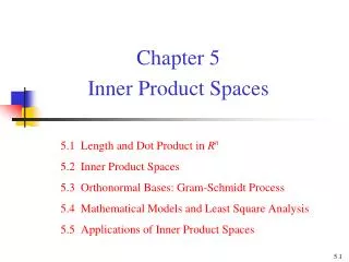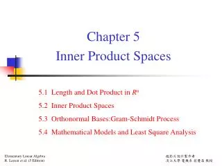
Chapter 7 Inner Product Spaces
490 likes | 1.28k Views
Linear Algebra. Chapter 7 Inner Product Spaces. 大葉大學 資訊工程系 黃鈴玲. Inner Product Spaces. In this chapter, we extend those concepts of R n such as: dot product of two vectors, norm of a vector, angle between vectors, and distance between points, to general vector space.

Chapter 7 Inner Product Spaces
E N D
Presentation Transcript
Linear Algebra Chapter 7Inner Product Spaces 大葉大學 資訊工程系 黃鈴玲
Inner Product Spaces • In this chapter, we extend those concepts of Rn such as: dot product of two vectors, norm of a vector, angle betweenvectors, and distance between points, to general vector space. • This will enable us to talk about the magnitudes of functionsand orthogonal functions. This concepts are used to approximate functions by polynomials – a technique that is used to implement functions on calculators and computers. • We will no longer be restricted to Euclidean Geometry,we will be able to create our own geometries on Rn.
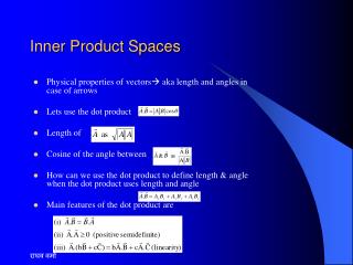
7.1 Inner Product Spaces The dot product was a key concept on Rn that led to definitions of norm,angle, and distance. Our approach will be to generalize the dot product of Rn to a general vector space with a mathematical structure called an innerproduct. This in turn will be used to define norm, angle, and distance fora general vector space.
Definition An inner product on a real spaces V is a function that associates a number, denoted 〈u, v〉, with each pair of vectors u and v of V. This function has to satisfy the following conditions for vectors u, v, and w, and scalar c. 1.〈u, v〉=〈v, u〉 (symmetry axiom) 2.〈u + v, w〉=〈u, w〉+〈v, w〉 (additive axiom) 3.〈cu, v〉= c〈u, v〉 (homogeneity axiom) 4.〈u, u〉 0, and 〈u, u〉= 0 if and only if u = 0 (position definite axiom) A vector space V on which an inner product is defined is called aninner product space. Any function on a vector space that satisfies the axioms of an inner productdefines an inner product on the space. There can be many inner products on a given vector space.
Example 1 Let u = (x1, x2), v = (y1, y2), and w = (z1, z2) be arbitrary vectors in R2. Prove that〈u, v〉, defined as follows, is an inner product on R2. 〈u, v〉= x1y1 + 4x2y2 Determine the inner product of the vectors (-2, 5), (3, 1) under this inner product. Solution Axiom 1:〈u, v〉= x1y1 + 4x2y2 = y1x1 + 4y2x2 =〈v, u〉 Axiom 2:〈u + v, w〉=〈 (x1, x2) + (y1, y2) , (z1, z2) 〉 =〈 (x1 + y1, x2 + y2), (z1, z2) 〉 = (x1 + y1) z1 + 4(x2 + y2)z2 = x1z1 + 4x2z2 + y1 z1 + 4 y2z2 =〈(x1, x2), (z1, z2)〉+〈(y1, y2), (z1, z2) 〉 =〈u, w〉+〈v, w〉
Axiom 4: 〈u, u〉= 〈(x1, x2), (x1, x2)〉= Further, if and only if x1 = 0 and x2 = 0. That is u = 0. Thus〈u, u〉 0, and〈u, u〉= 0 if and only if u = 0. The four inner product axioms are satisfied, 〈u, v〉= x1y1 + 4x2y2 is an inner product on R2. Axiom 3:〈cu, v〉= 〈c(x1, x2), (y1, y2)〉 =〈 (cx1, cx2), (y1, y2) 〉 = cx1y1 + 4cx2y2 = c(x1y1 + 4x2y2) = c〈u, v〉 The inner product of the vectors (-2, 5), (3, 1) is 〈(-2, 5), (3, 1)〉= (-2 3) + 4(5 1) = 14
Example 2 Consider the vector space M22 of 2 2 matrices. Let u and v defined as follows be arbitrary 2 2 matrices. Prove that the following function is an inner product on M22. 〈u, v〉= ae + bf + cg + dh Determine the inner product of the matrices . Solution Axiom 1:〈u, v〉= ae + bf + cg + dh = ea + fb + gc + hd =〈v, u〉 Axiom 3: Let k be a scalar. Then 〈ku, v〉= kae + kbf + kcg + kdh = k(ae + bf + cg + dh) = k〈u, v〉
Axiom 1: Axiom 2: Example 3 Consider the vector space Pn of polynomials of degree n. Let f and g be elements of Pn. Prove that the following function defines an inner product of Pn. Determine the inner product of polynomials f(x) = x2 + 2x – 1 and g(x) = 4x + 1 Solution
We now find the inner product of the functions f(x) = x2 + 2x – 1 and g(x) = 4x + 1
The norm of a vector in Rn can be expressed in terms of the dot product as follows Definition Let V be an inner product space. The norm of a vector v is denoted ||v|| and it defined by Norm of a Vector Generalize this definition: The norms in general vector space do not necessary have geometric interpretations, but are often important in numerical work.
The norm of the function f(x) = 5x2 + 1 is Example 4 Consider the vector space Pn of polynomials with inner product The norm of the function f generated by this inner product is Determine the norm of the function f(x) = 5x2 + 1. Solution Using the above definition of norm, we get
Example 2’ (補充) Consider the vector space M22 of 2 2 matrices. Let u and v defined as follows be arbitrary 2 2 matrices. It is known that the function 〈u, v〉= ae + bf + cg + dh is an inner product on M22 by Example 2. The norm of the matrix is
Definition Let V be an inner product space. The angle between two nonzero vectors u and v in V is given by Angle between two vectors The dot product in Rn was used to define angle between vectors. The angle between vectors u and v in Rn is defined by
Example 5 Consider the inner product space Pn of polynomials with inner product The angle between two nonzero functions f and g is given by Determine the cosine of the angle between the functions f(x) = 5x2 and g(x) = 3x Solution We first compute ||f || and ||g||. Thus
Example 2” (補充) Consider the vector space M22 of 2 2 matrices. Let u and v defined as follows be arbitrary 2 2 matrices. It is known that the function 〈u, v〉= ae + bf + cg + dh is an inner product on M22 by Example 2. The norm of the matrix is The angle between u and v is
Example 6 Show that the functions f(x) = 3x – 2 and g(x) = x are orthogonal in Pn with inner product Solution Thus the functions f and g are orthogonal in this inner product Space. Orthogonal Vectors Def. Let V be an inner product space. Two nonzero vectors u and v in V are said to be orthogonal if
Definition Let V be an inner product space with vector norm defined by The distance between two vectors (points) u and v is defined d(u,v) and is defined by Distance As for norm, the concept of distance will not have direct geometrical interpretation. It is however, useful in numerical mathematics to be able to discuss how far apart various functions are.
Thus The distance between f and h is 4, as we might suspect, g is closer than h to f. Example 7 Consider the inner product space Pn of polynomials discussed earlier. Determine which of the functions g(x) = x2 – 3x + 5 or h(x) = x2 + 4 is closed to f(x) = x2. Solution
Inner Product on Cn For a complex vector space, the first axiom of inner product is modified to read . An inner product can then be used to define norm, orthogonality, and distance, as far a real vector space. Let u = (x1, …, xn) and v = (y1, …, yn) be element of Cn. The most useful inner product for Cn is
Example 8 Consider the vectors u = (2 + 3i, -1 + 5i), v = (1 + i, -i) in C2. Compute (a)〈u, v〉, and show that u and v are orthogonal. (b) ||u|| and ||v|| (c) d(u, v) Solution
Homework • Exercise 7.1:1, 4, 8(a), 9(a), 10, 12, 13, 15, 17(a), 19, 20(a)
Example Let u = (x1, x2), v = (y1, y2) be arbitrary vectors in R2. It is proved that〈u, v〉, defined as follows, is an inner product on R2. 〈u, v〉= x1y1 + 4x2y2 7.2 Non-Euclidean Geometry and Special Relativity Different inner products on Rn lead to different measures of vector norm, angle, and distance – that is, to different geometries. dot product Euclidean geometryother inner products non-Euclidean geometries The inner product differs from the dot product in the appearance of a 4. Consider the vector (0, 1) in this space. The norm of this vector is
Figure 7.1 The norm of this vector in Euclidean geometry is 1;in our new geometry, however, the norm is 2.
Figure 7.2 Consider the vectors (1, 1) and (-4, 1). The inner product of these vectors is Thus these two vectors are orthogonal.
Figure 7.3 Let us use the definition of distance based on this inner product to compute the distance between the points(1, 0) and (0, 1). We have that
7.4 Least-Squares Curves To find a polynomial that best fits given data points. Ax = y : (1) if n equations, n variables, and A-1 exists x = A-1y(2) if n equations, m variables with n > m overdetermined How to solve it? We will introduce a matrix called the pseudoinverse of A, denoted pinv(A), that leads to a least-squares solutionx = pinv(A)y for an overdetermined system.
Example 1 Find the pseudoinverse of A = Solution Definition Let A be a matrix. The matrix (AtA)-1At is called the pseudoinverse of A and is denoted pinv(A).
Let Ax = ybe a system of n linear equations in m variables with n > m, where A is of rank m. Ax=y AtAx=Aty x = (AtA)-1Aty AtA is invertible Ax = yx = pinv(A)y system least-squares solution If the system Ax=y has a unique solution, the least-squares solution is that unique solution. If the system is overdetermined, the least-squares solution is the closest we can get to a true solution. The system cannot have many solutions.
The matrix of coefficients is Example 2 Find the least-squares solution of the following overdetermined system of equations. Sketch the solution. Solution rank(A)=2
Figure 7.9 The least-squares solution is The least-squares solution is the point
Least-Square Curves Least-squares line or curve minimizes Figure 7.10
Let the equation of the line by y = a + bx. Substituting for these points into the equation of the line, we get the overdetermined system We find the least squares solution. The matrix of coefficients A and column vector y are as follows. It can be shown that Example 3 Find the least-squares line for the following data points. (1, 1), (2, 4), (3, 2), (4, 4) Solution
Figure 7.11 The least squares solution is Thus a = 1, b = 0.7. The equation of the least-squares line for this data is y = 1 + 0.7x
Let the equation of the parabola be y = a + bx + cx2. Substituting for these points into the equation of the parabola, we get the system We find the least squares solution. The matrix of coefficients A and column vector y are as follows. It can be shown that Example 4 Find the least-squares parabola for the following data points. (1, 7), (2, 2), (3, 1), (4, 3) Solution
Figure 7.12 The least squares solution is Thus a = 15.25, b = -10.05, c = 1.75. The equation of the least-squares parabola for these data points is y = 15.25 – 10.05x + 1.75x2
Theorem 7.1 Let (x1, y1), …, (xn, yn) be a set of n data points. Let y = a0 + … + amxm be a polynomial of degree m (n > m) that is to be fitted to these points. Substituting these points into the polynomial leads to a system Ax = y of n linear equations in the m variables a0, …, am, where The least-squares solution to this system gives the coefficients of the least-squares polynomial for these data points. Figure 7.13 y’ is the projection of y onto range(A)
Homework • Exercise 7.43, 11, 21