Hough Transform (Section 10.2)
Hough Transform (Section 10.2). CS474/67. Edge Linking and Boundary Detection. Edge detection does not yield connected boundaries. Edge linking and boundary following must be applied after edge detection. thresholded gradient magnitude. gradient magnitude. Local Processing Methods.

Hough Transform (Section 10.2)
E N D
Presentation Transcript
Hough Transform (Section 10.2) CS474/67
Edge Linking and Boundary Detection • Edge detection does not yield connected boundaries. • Edge linking and boundary following must be applied after edge detection. thresholded gradient magnitude gradient magnitude
Local Processing Methods • At each pixel, a neighborhood (e.g., 3x3) is examined. • Pixels which are similar in this neighborhood are linked. • How do we define similarity ?
Local Processing Methods (cont’d) Gx - Sobel Gy - Sobel linking results T=25, A=15
Global Processing Methods • If gaps are very large, local processing methods are not effective. • Model-based approaches can be used in this case! • Hough Transform can be used to determine whether points lie on a curve of a specified shape.
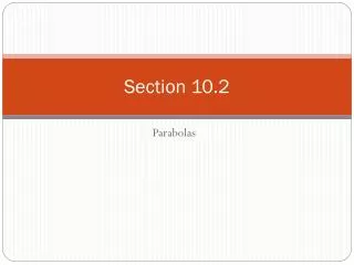
Hough Transform – Line Detection • Consider the slope-intercept equation of line • Rewrite the equation as follows (a, b are constants, x is a variable, y is a function of x) (now, x, y are constants, a is a variable, b is a function of a)
Hough Transform – Line Detection (cont’d) x-y space slope-intercept space
Properties in slope-intercept space • Each point (xi, yi) defines a line in the a − b space (parameter space). • Points lying on the same line in the x − y space, define lines in the parameter space which all intersect at the same point. • The coordinates of the point of intersection define the parameters of the line in the x − y space.
Algorithm 1. Quantize parameter space (a,b): P[amin, . . . , amax][bmin, . . . , bmax] (accumulator array) amax
Algorithm (cont’d) 2. For each edge point (x, y) For(a = amin; a ≤ amax; a++) { b = − xa + y; /* round off if needed * (P[a][b])++; /* voting */ } 3. Find local maxima in P[a][b] if P[a j][bk]=M, then M points lie on the line y = a j x + bk
Effects of Quantization • The parameters of a line can be estimated more accurately using a finer quantization of the parameter space. • Finer quantization increases space and time requirements. • For noise tolerance, however, a coarser quantization is better. amax
Problems with slope-intercept equation • The slope can become very large or even infinity! • e.g., for vertical or close to vertical lines • Suppose (x1,y1) and (x2,y2) lie on the line: • It will be impossible to quantize such a large space! slope:
Polar Representation of Lines (no problem with vertical lines, i.e., θ =90) ρ−θ space
Properties in ρ−θ space • Each point (xi, yi) defines a sinusoidal curve in the ρ −θ space (parameter space). • Points lying on the same line in the x − y space, define lines in the parameter space which all intersect at the same point. • The coordinates of the point of intersection define the parameters of the line in the x − y space.
Properties in ρ−θ space (cont’d) D: max distance ρ=√2D -ρ=-√2D
Example long vertical lines
Algorithm 1. Quantize the parameter space (ρ,θ) P[ρmin, . . . , ρmax][θmin, . . . ,θmax] (accumulator array)
Algorithm (cont’d) 2. For each edge point (x, y) For(θ = θmin;θ ≤ θmax;θ ++) { ρ = xcos(θ) + ysin(θ) ; /* round off if needed * (P[ρ][θ])++; /* voting */ } 3. Find local maxima in P[ρ][θ]
Example Richard Duda and Peter Hart “Use of the Hough Transformation to Detect Lines and Curves in Pictures” Communications of the ACM Volume 15 , Issue 1 (January 1972) Pages: 11 – 15
Extending Hough Transform • Hough transform can also be used for detecting circles, ellipses, etc. • For example, the equation of circle is: • In this case, there are three parameters: (x0, y0), r
Extending Hough Transform (cont’d) • In general, we can use hough transform to detect any curve which can be described analytically by an equation of the form: • Detecting arbitrary shapes, with no analytical description, is also possible (i.e., Generalized Hough Transform)