HOUGH TRANSFORM
HOUGH TRANSFORM. Presentation by Sumit Tandon Department of Electrical Engineering University of Texas at Arlington Course # EE6358 Computer Vision. Contents. Introduction Advantages of Hough transform Hough Transform for Straight Line Detection Hough Transform for Circle Detection

HOUGH TRANSFORM
E N D
Presentation Transcript
HOUGH TRANSFORM Presentation by Sumit Tandon Department of Electrical Engineering University of Texas at Arlington Course # EE6358 Computer Vision
Contents • Introduction • Advantages of Hough transform • Hough Transform for Straight Line Detection • Hough Transform for Circle Detection • Recap and list of parameters • Generalized Hough Transform • Improvisation of Hough Transform • Examples • References EE6358 - Computer Vision
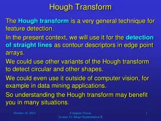
1. Introduction • Performed after Edge Detection • It is a technique to isolate the curves of a given shape / shapes in a given image • Classical Hough Transform can locate regular curves like straight lines, circles, parabolas, ellipses, etc. • Requires that the curve be specified in some parametric form • Generalized Hough Transform can be used where a simple analytic description of feature is not possible EE6358 - Computer Vision
2. Advantages of Hough Transform • The Hough Transform is tolerant of gaps in the edges • It is relatively unaffected by noise • It is also unaffected by occlusion in the image EE6358 - Computer Vision
3.1 Hough Transform for Straight Line Detection • A straight line can be represented as • y = mx + c • This representation fails in case of vertical lines • A more useful representation in this case is • Demo EE6358 - Computer Vision
3.2 Hough Transform for Straight Lines • Advantages of Parameterization • Values of ‘r’ and ‘q’ become bounded • How to find intersection of the parametric curves • Use of accumulator arrays – concept of ‘Voting’ • To reduce the computational load use Gradient information EE6358 - Computer Vision
3.3 Computational Load • Image size = 512 X 512 • Maximum value of • With a resolution of 1o, maximum value of • Accumulator size = • Use of direction of gradient reduces the computational load by 1/360 EE6358 - Computer Vision
3.4 Hough Transform for Straight Lines - Algorithm • Quantize the Hough Transform space: identify the maximum and minimum values of r and q • Generate an accumulator array A(r, q); set all values to zero • For all edge points (xi, yi) in the image • Use gradient direction for q • Compute r from the equation • Increment A(r, q) by one • For all cells in A(r, q) • Search for the maximum value of A(r, q) • Calculate the equation of the line • To reduce the effect of noise more than one element (elements in a neighborhood) in the accumulator array are increased EE6358 - Computer Vision
3.5 Line Detection by Hough Transform EE6358 - Computer Vision
4.1 Hough Transform for Detection of Circles • The parametric equation of the circle can be written as • The equation has three parameters – a, b, r • The curve obtained in the Hough Transform space for each edge point will be a right circular cone • Point of intersection of the cones gives the parameters a, b, r EE6358 - Computer Vision
4.2 Hough Transform for Circles • Gradient at each edge point is known • We know the line on which the center will lie • If the radius is also known then center of the circle can be located EE6358 - Computer Vision
4.3 Detection of circle by Hough Transform - example Original Image Circles detected by Canny Edge Detector EE6358 - Computer Vision
4.4 Detection of circle by Hough Transform - contd Hough Transform of the edge detected image Detected Circles EE6358 - Computer Vision
5.1 Recap • In detecting lines • The parameters r and q were found out relative to the origin (0,0) • In detecting circles • The radius and center were found out • In both the cases we have knowledge of the shape • We aim to find out its location and orientation in the image • The idea can be extended to shapes like ellipses, parabolas, etc. EE6358 - Computer Vision
5.2 Parameters for analytic curves EE6358 - Computer Vision
6.1 Generalized Hough Transform • The Generalized Hough transform can be used to detect arbitrary shapes • Complete specification of the exact shape of the target object is required in the form of the R-Table • Information that can be extracted are • Location • Size • Orientation • Number of occurrences of that particular shape EE6358 - Computer Vision
6.2 Creating the R-table • Algorithm • Choose a reference point • Draw a vector from the reference point to an edge point on the boundary • Store the information of the vector against the gradient angle in the R-Table • There may be more than one entry in the R-Table corresponding to a gradient value EE6358 - Computer Vision
6.3 Generalized Hough Transform - Algorithm • Form an Accumulator array to hold the candidate locations of the reference point • For each point on the edge • Compute the gradient direction and determine the row of the R-Table it corresponds to • For each entry on the row calculate the candidate location of the reference point • Increase the Accumulator value for that point • The reference point location is given by the highest value in the accumulator array EE6358 - Computer Vision
6.4 Generalized Hough Transform – Size and Orientation • The size and orientation of the shape can be found out by simply manipulating the R-Table • For scaling by factor S multiply the R-Table vectors by S • For rotation by angle q, rotate the vectors in the R-Table by angle q EE6358 - Computer Vision
6.5 Generalized Hough Transform – Advantages and disadvantages • Advantages • A method for object recognition • Robust to partial deformation in shape • Tolerant to noise • Can detect multiple occurrences of a shape in the same pass • Disadvantages • Lot of memory and computation is required EE6358 - Computer Vision
7.1 Improvisation of the Hough transform for detecting straight line segments • Hough Transform lacks the ability to detect the end points of lines – localized information is lost during HT • Peak points in the accumulator can be difficult to locate in presence of noisy or parallel edges • Efficiency of the algorithm decreases if image becomes too large • New approach is proposed to reduce these problems EE6358 - Computer Vision
7.2 Spatial decomposition • This technique preserves the localized information • Divide the image recursively into quad-trees, each quad-tree representing a part of the image i.e. a sub-image • The leaf nodes will be voted for feature points which are in the sub-image represented by the leaf node EE6358 - Computer Vision
7.2 Spatial Decomposition of Hough Transform • Parameter space is defined from a global origin rather than a local one • Each node contains information about the sub-nodes as well as the number of feature points in the sub-image represented by the node • Pruning of sub-trees is done if the number of the feature points falls below a threshold • An accumulator is assigned for each leaf node EE6358 - Computer Vision
7.3 Some relations involved in spatial decomposition • Consider the following • Q – any non-leaf node • F – feature points in the sub-image represented by this node • A – parameter space of the sub-image • The following relations hold true EE6358 - Computer Vision
7.4 Number of accumulator arrays required • Consider the following case • Size of image = N X N • Size of leaf node = M X M • Depth of tree = d (root node = 0) • Number of accumulator arrays for only leaf nodes = • Number of accumulator arrays for all nodes = EE6358 - Computer Vision
7.5 Example EE6358 - Computer Vision
References • Generalizing The Hough Transform to Detect Arbitrary Shapes – D H Ballard – 1981 • Spatial Decomposition of The Hough Transform – Heather and Yang – IEEE computer Society – May 2005 • Hypermedia Image Processing Reference 2 – http://homepages.inf.ed.ac.uk/rbf/HIPR2/hipr_top.htm • Machine Vision – Ramesh Jain, Rangachar Kasturi, Brian G Schunck, McGraw-Hill, 1995 • Machine Vision - Wesley E. Snyder, Hairong Qi, Cambridge University Press, 2004 EE6358 - Computer Vision