Download

1 / 38
380 likes | 536 Views
Aspects of Transitional flow for External Applications. A review presented by Clare Turner. Presentation Outline. Review of T3 flat plate tests. Conclusions from the flat plate tests. Direction for transition prediction. Current and future work. T3 Flat Plate Tests.

E N D
Aspects of Transitional flow for External Applications A review presented by Clare Turner
Presentation Outline • Review of T3 flat plate tests • Conclusions from the flat plate tests • Direction for transition prediction • Current and future work
Original Simulation Set-up • Domain size taken from S. R. Likki : • S = 0.05m • L = 3.3m • H = 0.08m • Inlet conditions: • k = 0.0536 m2/s2 • ε = 1.35 m2/s3 • U = 5.08 m/s • y+ ≈ 1
Anomalous Results After Craft et al.:
Possible Areas for Error • Differencing scheme • Grid density • y+ value • Residual tolerance • Domain size • Boundary conditions • Cell distribution • Near wall treatment
Number of cross-stream cells • Grids have 23, 34 and 39 cells in the viscous layer respectively
Cell Distribution • Several meshes generated to compare results and convergence; largest cell distribution: • More efficient to concentrate cells at the leading edge • 39390
Convergence To the left: growthrate=1; to the right growthrate = 1.012
Low Reynolds Number Models Available in Star-CD: “Standard” where
Low Reynolds Number Models Available in Star-CD: Suga’s where
Determination of Inlet Values • Dissipation rate originally tailored to FSTI curve
Re-calibration of Inlet Values • Free-stream taken to be at the edge of boundary layer • Experimentally free-stream is at approximately 3 delta • Turbulence intensities calculated with new definition
Effect of Chosen Free-stream boundary • Error was not in the calculation of the free-stream
Inlet Values in Literature • Inlet k and epsilon values differ to those in literature • Differences may arise due to choice of U_inlet • 3 different inlets are tested with U = 5 m/s: • Using a correlation for lengthscale from work of Savill and interpolating FSTI at inlet • As above but with a higher FSTI • As 2) but with a lengthscale used by Chen et al.
Choice of Inlet Velocity • Original velocity set to 5.08 • Velocity at leading edge should be approx 5 m/s • Turbulence model does not replicate acceleration at the leading edge
T3 Conclusions • Largest contributing factor is the low Reynolds number treatment • Sufficient work has been done on the grid to only require small alterations for future tests • Non-linear eddy-viscosity models improve transition onset prediction and running time is not increased dramatically but no alterations can improve transition length prediction.
Approaches for a Physical Solution rather than Correlation Based Models 3 possible approaches: Adaptation of low Reynolds number RANS models, eg. higher order of closure, tailored to specific application. An intermittency model derived using PDFs A model using the concept of laminar kinetic energy
1) Low Reynolds Number RANS Models Advantages: Large amount of in-house knowledge Have models to develop, low risk Disadvantages: Nothing new to contribute Low Re models do not accurately represent the transition process Higher orders of closure increase computational cost
2) Physical Intermittency Model Advantages: New approach Should be able to predict all modes of transition Disadvantages: No literature to refer to - risky Have little expertise in PDFs Little or no time would remain to apply to rear wing
3) Concept of Laminar Kinetic Energy Advantages: Relatively new giving areas for improvement Does not rely on diffusion dominated transition Only requires one additional equation Disadvantages: Walters and Leylek model (2002) gives poor reaction to large pressure gradients Determination of the effective length-scale is only based on distance from the wall
Walters and Leylek Model (2003) • This is the starting point for 2k model development
Walters and Leylek Model (2003) • Walters and Leylek assume large scales contribute to the laminar kinetic energy and small scales to the turbulent kinetic energy. • The cut – off point is the effective length-scale : • Sveningsson uses a different definition:
Effective Length-scale Along the Plate At 400 mm (transitional region) : δ99 = 18.5 mm
Effective Length-scale Along the Plate At 800 mm (turbulent region) : δ99 = 24.1 mm
Current Work • Adjusting individual terms of Wilcox’s transport equations for turbulent kinetic energy and specific dissipation rate to those of Walters and Leylek • Testing code by inserting fully turbulent values from completed simulations Aiming to ... • Use code with Saturne assuming laminar kinetic energy = 0 • Create new scalar variable KL to complete Walters and Leylek Model