Fast and accurate text classification via multiple linear discriminant projections

1. Fast and accurate text classification via multiple linear discriminant projections Soumen ChakrabartiShourya RoyMahesh Soundalgekar IIT Bombay www.cse.iitb.ac.in/~soumen

2. Introduction • Supervised learning of labels from high-dimensional data has many applications • Text topic and genre classification • Many classification algorithms known • Support vector machines (SVM)—most accurate • Maximum entropy classifiers • Naïve Bayes classifiers—fastest and simplest • Problem: SVMs • Are difficult to understand and implement • Take time almost quadratic in #instances

3. Our contributions • Simple Iterated Multiple Projection on Lines (SIMPL) • Trivial to understand and code (600 lines) • O(#dimensions) or less memory • Only sequential scans of training data • Almost as fast as naïve Bayes (NB) • As accurate as SVMs, sometimes better • Insights into the best choice of linear discriminants for text classification • How do the discriminants chosen by NB, SIMPL and SVM differ?

4. Naïve Bayes classifiers • For simplicity assume two classes {1,1} • t=term, d=document, c=class, d=length of document d, n(d,t)=#times t occurs in d • Model parameters • Priors Pr(c=1) and Pr(c=1) • c,t=fractional rate at which t occurs in documents labeled with class c • Probability of a given d generated from c is

5. Naïve Bayes is a linear discriminant • When choosing between the two labels • Terms involving document length cancel out • Taking logs, we compare • The first part is a dot-product, the second part is a fixed offset, so we compare • Simple join-aggregate, very fast

6. Many features, each fairly noisy • Sort features in order ofdecreasing correlationwith class labels • Build separate classifiers • 1—100, 101—200, etc. • Even features ranked5000 to 10000 providelift beyond picking arandom class • Most features have tiny amounts of useful, noisy and possibly redundant info—how to combine? • Naïve Bayes, LSVM, maximum entropy—all take linear combinations of term frequencies

7. All traininginstanceshere havec=1 d1 d2  All traininginstanceshere havec= 1 d+b=1 d+b=0 d+b=1 Support vector Linear support vector machine (LSVM) • Want a vector  and a constant b such that for each document di • If ci=1 then di+b  1 • If ci=1 then di+b  1 • I.e., ci(di+b)  1 • If points d1 and d2touch the slab, the projected distance between them is • Find  to maximize this

8. SVM implementations • SVM is a linear sum of support vectors • Complex, non-linear optimization • 6000 lines of C code (SVM-light) • Approx n1.7—1.9 time with n training vectors • Footprint can be large • Usually hold all training vectors in memory • Also a cache of dot-products of vector pairs • No I/O-optimized implementation known • We measured 40% time in seek+transfer

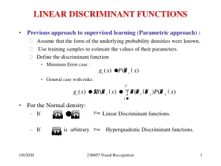
9. Square of distance between projectedmeans Variance of projected X-points Variance of projected Y-points Fisher’s linear discriminant (FLD) • Used in pattern recognition for ages • Two point sets X (c=1) and Y (c=1) • xX, yY are points in m dimensions • Projection on unit vector  is x · , y ·  • Goal is to find a direction  so as to maximize

10. Some observations • Hyperplanes can often completely separate training labels for text; more complex separators do not help (Joachims) • NB is biased: tdepends only on term t—SVM/Fisher do not make this assumption • If you find Fisher’s discriminant over only the support vectors, you get the SVM separator (Shashua) • Even random projections preserve inter-point distances whp (Frankl+Maehara 1988, Kleinberg 1997)

11. Hill-climbing • Iteratively update newold + J() where  is a “learning rate” • J() = (J/1,…,J/m)T where  = (1,…,m)T • Need only 5m + O(1) accumulators for simple, one-pass update • Can also write as sort-merge-accumulate

12. Convergence • Initialize  to vectorjoining positive and negative centroids • Stop if J() cannot be increased in three successive iterations • J() converges in10—20 iterations • Not sensitiveto problem size • 120000 documents from http://dmoz.org • LSVM takes 20000 seconds • Hill-climbing converges in 200 seconds

13. Confusion zone Multiple discriminants • Separable data points • SVM succeeds • FLD fails to separate completely • Idea • Remove training points (outside the gray zone) • Find another FLD for surviving points only • 2—3 FLDs suffice for almost complete separation! • 70742302

14. SIMPL (only 600 lines of C++) • Repeat for k = 0, 1, … • Find (k), the Fisher discriminant for the current set of training instances • Project training instances to (k) • Remove points well-separated by (k) • while 1 point from each class survive • Orthogonalize the vectors (0),(1), (2),… • Project all training points on the space spanned by the orthogonal ’s • Induce decision tree on projected points

15. Robustness of stopping decision • Compute (0) to convergence • Vs., run only half the iterations required for convergence • Find (1),… as usual • Later s can cover for slop in earlier s • While saving time in costly early- updates • Later s take negligible time

16. Accuracy • Large improvement beyond naïve Bayes • We tuned parameters in SVM to give “SVM-best” • Often beats SVM with default params • Almost always within 5% of SVM-best • Even beats SVM-best in some cases • Especially when problem is not linearly separable

17. SVM SIMPL is linear-time and CPU-bound LSVM spends 35—60% time in I/O+cache mgmt LSVM takes 2 orders of magnitude more time for 120000 documents Performance

18. Summary and future work • SIMPL: a new classifier for high-dimensional data • Low memory footprint, sequential scan • Orders of magnitude faster than LSVM • Often as accurate as LSVM, sometimes better • An efficient “feature space transformer” • How will SIMPL behave for non-textual, high-dim data? • Can we analyze SIMPL? • LSVM is theoretically sound, more general • When will SIMPL match LSVM/SVM?