
Patterns matching
E N D
Presentation Transcript
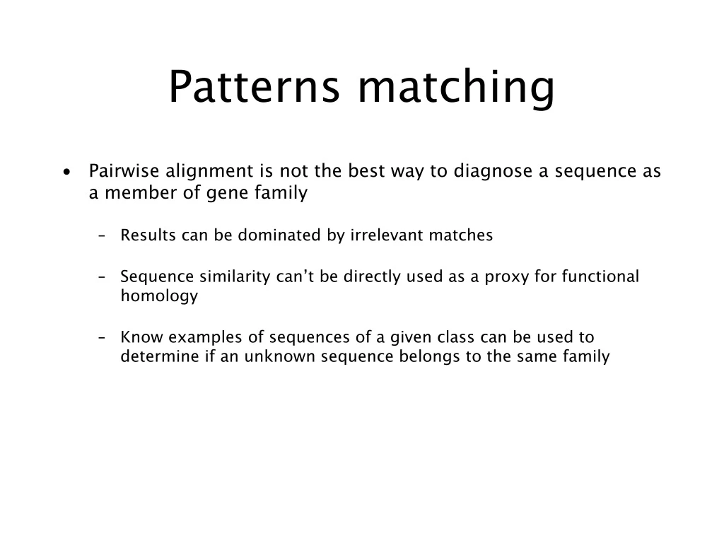
Patterns matching • Pairwise alignment is not the best way to diagnose a sequence as a member of gene family • Results can be dominated by irrelevant matches • Sequence similarity can’t be directly used as a proxy for functional homology • Know examples of sequences of a given class can be used to determine if an unknown sequence belongs to the same family
Pattern • A pattern can be more or less anything that is unique to the sequences of the class of interest. • Patterns describe features that are common to all member of the class. • Patterns have to be sufficiently flexible to account for some degree of variation.
A good method should have high sensitivity, i.e., it should correctly identify as many true-positive members of the family as possible. • It should also have high selectivity, i.e., very few false-positive sequences should be incorrectly predicted to be members of the family
Position specific scoring matrix (PSSM) • Matching any given amino acid at a given position. • Not only matching is important, but also where (which position) the matching is also is important.
Three different methods • Regular expressions • Fingerprints • Blocks
Regular expressions (regexs) • The simplest pattern-recognition method • Used by PROSITE (Falquet et al. 2002)
Fingerprint • Used in PRINTS (Attwood et al., 2003)
Its diagnostic power is refined by iterative scanning of a SWISS-PROT/TrEMBL. • Full diagnostic potency deriving from the mutual context provided by motif neighbours.
Blocks • BLOCKS database • Reduce multiple contribution to residue frequencies from groups of closely related sequences. • Each cluster is treated as a single segment and assigned a weight
Profiles • By contrast with motif-base pattern-recognition techniques, an alternative approach is to distil the sequence information within complete alignments into scoring tables, or profiles. • Help in diagnostic sequences with high divergence.
Applications • Speech recognition • Machine translation • Gene prediction • Sequences alignment • Time Series Analysis • Protein folding • …
Markov Model • A system with states that obey the Markov assumption is called a Markov Model • A sequence of states resulting from such a model is called a Markov Chain.
Hidden Markov model • A hidden Markov model (HMM) is a statistical Markov model in which the system being modeled is assumed to be a Markov process with unobserved (hidden) states.
Notice that only the observations y are visible, the states x are hidden to the outside. This is where the name Hidden Markov Models comes from
Hidden Markov Models • Components: • Observed variables • Emitted symbols • Hidden variables • Relationships between them • Represented by a graph with transition probabilities • Goal: Find the most likely explanation for the observed variables
The occasionally dishonest casino • A casino uses a fair die most of the time, but occasionally switches to a loaded one • Fair die: Prob(1) = Prob(2) = . . . = Prob(6) = 1/6 • Loaded die: Prob(1) = Prob(2) = . . . = Prob(5) = 1/10, Prob(6) = ½ • These are the emission probabilities • Transition probabilities • Prob(Fair Loaded) = 0.01 • Prob(Loaded Fair) = 0.2 • Transitions between states obey a Markov process
The occasionally dishonest casino • Known: • The structure of the model • The transition probabilities • Hidden: What the casino did • FFFFFLLLLLLLFFFF... • Observable: The series of die tosses • 3415256664666153... • What we must infer: • When was a fair die used? • When was a loaded one used? • The answer is a sequenceFFFFFFFLLLLLLFFF...
Making the inference • Model assigns a probability to each explanation of the observation: P(326|FFL) = P(3|F)·P(FF)·P(2|F)·P(FL)·P(6|L) = 1/6 · 0.99 · 1/6 · 0.01 · ½ • Maximum Likelihood: Determine which explanation is most likely • Find the path most likely to have produced the observed sequence • Total probability: Determine probability that observed sequence was produced by the HMM • Consider all paths that could have produced the observed sequence
Notation • xisthe sequence of symbols emitted by model • xiis the symbol emitted at time i • A path, , is a sequence of states • The i-th state in is i • akr is the probability of making a transition from state k to state r: • ek(b) is the probability that symbol b is emitted when in state k
0 0 1 1 1 1 … 2 2 2 2 … … … … … K K K K … A “parse” of a sequence 1 2 2 K x1 x2 x3 xL
The most probable path The most likely path * satisfies To find *, consider all possible ways the last symbol of x could have been emitted Let Then
The Viterbi Algorithm • Initialization (i = 0) • Recursion (i = 1, . . . , L): For each state k • Termination: To find *, use trace-back, as in dynamic programming
Viterbi: Example x 2 6 6 0 0 B 1 0 (1/6)max{(1/12)0.99, (1/4)0.2} = 0.01375 (1/6)max{0.013750.99, 0.020.2} = 0.00226875 (1/6)(1/2) = 1/12 0 F (1/2)max{0.013750.01, 0.020.8} = 0.08 (1/10)max{(1/12)0.01, (1/4)0.8} = 0.02 (1/2)(1/2) = 1/4 0 L
Total probabilty Many different paths can result in observation x. The probability that our model will emit x is Total Probability If HMM models a family of objects, we want total probability to peak at members of the family. (Training)
å f ( i ) e ( x ) f ( i 1 ) a = - r i k k rk r Total probabilty Pr(x) can be computed in the same way as probability of most likely path. Let Then and
The Forward Algorithm • Initialization (i = 0) • Recursion (i = 1, . . . , L): For each state k • Termination:
Estimating the probabilities (“training”) • Baum-Welch algorithm • Start with initial guess at transition probabilities • Refine guess to improve the total probability of the training data in each step • May get stuck at local optimum • Special case of expectation-maximization (EM) algorithm • Viterbi training • Derive probable paths for training data using Viterbi algorithm • Re-estimate transition probabilities based on Viterbi path • Iterate until paths stop changing
Profile HMMs • Model a family of sequences • Derived from a multiple alignment of the family • Transition and emission probabilities are position-specific • Set parameters of model so that total probability peaks at members of family • Sequences can be tested for membership in family using Viterbi algorithm to match against profile
Profile HMMs: Example Note: These sequences could lead to other paths.
A Characterization Example How could we characterize this (hypothetical) family of nucleotide sequences? • Keep the Multiple Alignment • Try a regular expression [AT] [CG] [AC] [ACTG]* A [TG] [GC] • But what about? • T G C T - - A G G vrs • A C A C - - A T C • Try a consensus sequence: A C A - - - A T C • Depends on distance measure Example borrowed from Salzberg, 1998
HMMs to the rescue! Emission Probabilities Transition probabilities
Scoring our simple HMM • #1 - “T G C T - - A G G” vrs: #2 - “A C A C - - A T C” • Regular Expression ([AT] [CG] [AC] [ACTG]* A [TG] [GC]): • #1 = Member #2: Member • HMM: • #1 = Score of 0.0023% #2 Score of 4.7% (Probability) • #1 = Score of -0.97 #2 Score of 6.7 (Log odds)
Pfam • “A comprehensive collection of protein domains and families, with a range of well-established uses including genome annotation.” • Each family is represented by two multiple sequence alignments and two profile-Hidden Markov Models (profile-HMMs). • A. Bateman et al. Nucleic Acids Research (2004) Database Issue 32:D138-D141
Biological Motivation: • Given a single amino acid target sequence of unknown structure, we want to infer the structure of the resulting protein.
But wait, that’s hard! • There’s physics, chemistry, secondary structure, tertiary structure and all sorts of other nasty stuff to deal with. • Let’s rephrase the problem: • Given a target amino acid sequence of unknown structure, we want to identify the structural family of the target sequence through identification of a homologous sequence of known structure.
It still sounds hard… • In other words: • We find a similar protein with a structure that we understand, and we see if it makes sense to fold our target into the same sort of shape. • If not, we try again with the second most similar structure, and so on. • What we’re doing is taking advantage of the wealth of knowledge that has been collected in protein and structure databases.