Download
1 / 25
250 likes | 363 Views
Variability of the Upper Troposphere and Lower Stratosphere ozone from assimilation and model. K.Wargan, I. Stajner, S. Pawson, L. Froidevaux, N. Livesey, and P. K. Bhartia. Questions to be addressed. How does data assimilation impact the structure/variability of the ozone field in the UTLS?

E N D
Variability of the Upper Troposphere and Lower Stratosphere ozone from assimilation and model K.Wargan, I. Stajner, S. Pawson, L. Froidevaux, N. Livesey, and P. K. Bhartia
Questions to be addressed • How does data assimilation impact the structure/variability of the ozone field in the UTLS? • How does the variability of assimilated ozone compare with that of high frequency aircraft data – the question of effective resolution
Motivation Some bad things that people say about data assimilation
Tom Birner’s ‘Asmoothilation’ effect July January CMAM Zonal mean TB-mean buoyancy frequency squared (10-4 s-2, color shading) and isentropes (contours, overworld dashed). T.Birner et al. G.R.L 33, 2006
Tom Birner’s ‘Asmoothilation’ effect July January CMAM Data Assimilation CMAM-DA 2002 Zonal mean TB-mean buoyancy frequency squared (10-4 s-2, color shading) and isentropes (contours, overworld dashed). T.Birner et al. G.R.L 33, 2006
Tom Birner’s ‘Asmoothilation’ effect July January Data Assimilation Harmless?!... CMAM Data Assimilation CMAM-DA 2002 Zonal mean TB-mean buoyancy frequency squared (10-4 s-2, color shading) and isentropes (contours, overworld dashed). T.Birner et al. G.R.L 33, 2006
…but that’s dynamical DA. What about assimilating constituents? Should we expect Undesirable smoothing effects? Spurious features?
Methodology • An assimilation run is compared with a model (all ozone data withheld) experiment • The two are compared with data from aircraft measurements (Mozaic) averaged to match the resolution of the model • Statistical comparisons are done in terms of ozone power spectra
Ozone assimilation system • MODEL • transport within GEOS-4 general circulation model constrained by meteorological analyses • parameterizations for stratospheric photochemistry and heterogeneous ozone loss • a parameterization of the tropospheric chemistry DATA • The Microwave Limb Sounder (MLS): ozone profiles: • 20 levels 216 – 0.14 hPa • ~ 3,500 profiles a day, near global coverage • Ozone Monitoring Instrument (OMI): US retrieved ozone total column (low reflectivity). Data averaged onto a 2°× 2.5° grid • Data input and analysis output every 3 hours • The model grid: 1°× 1.25° × 55 levels
Tracer field structure. A case study Assimilation Model An ozone-rich filament extends from N. America down to the tropics. This feature is seen in both, model and assimilation runs. Morphology of the field is determined by the model (a) (b) Ozone mixing ratio [ppmv] at 118.25 hPa on March 16th 2005, 6 UTC from (a) assimilation and (b) model
Tracer field structure. A case study Model Assimilation Model and assimilation produce the same number of local minima and maxima at roughly the same locations… Ozone mixing ratio at 118.25 hPa along the 40°N latitude circle on March 16th 2005, 6 UTC from assimilation (green) and model (black).
Tracer field structure. A case study Model Assimilation …but the field values and amplitudes may be different
March 2005 July 2005 Assimilation vs aircraft Assimilation vs aircraft Model vs aircraft Model vs aircraft Assimilation expected to generate larger amplitudes than model Model expected to generate larger amplitudes than assimilation Assimilation acts on modes of tracer distribution Ozone [ppmv] Ozone [ppmv]
Variability in terms of power spectra Power spectra of ozone mixing ratio are calculated from 4000 km long flight segments and interpolated model/analysis Mozaic Model Assimilation July large small 4000 1000 400 200 [km] • Variability is underestimated in model and analysis • Higher amplitudes in assimilation are likely a reflection of bias correction in the stratosphere
Variability in terms of power spectra Mozaic Model Assimilation March July large small large small 4000 1000 400 200 [km] 4000 1000 400 200 [km] • In March the opposite is true: stratospheric ozone in assimilation is lower than in model yielding smaller amplitudes
Variability in terms of power spectra Mozaic/assim Model/assim March July large small large small 4000 1000 400 200 [km] 4000 1000 400 200 [km] • In all months, analysis and model spectra appear to have the same slope
Resolution vs effective resolution smoothing Smoothing the aircraft data Causes the aircraft power spectrum to collapse onto that calculated from the model. The value of n = 4 is used here: smoothing over 5 grid-cells 4000 1000 400 [km]
Summary of results so far • No evidence of smoothing or roughening effects of assimilation. Field structure determined by model • Model unable to resolve tracer variability at small scales
Interpretation Analysis increments are an order of magnitude smaller than transport increments. Advection does not generate new maxima or minima. At small scales numerical diffusion kicks in. Advection transfers tracer variability downscales from large basins Ratio of monthly zonal RMS of transport to analysis increments at 192.5 hPa pressure level in July 2005
Interpretation SBUV+POAM SBUV Analysis increments are an order of magnitude smaller than transport increments. Advection does not generate new maxima or minima. At small scales numerical diffusion kicks in. Advection transfers tracer variability downscales from large basins Ozone mixing ratio (in ppmv) at 70 hPa on three days in year 1998: August 1 (a and b), September 1 (c and d), and October 20 (e and f). Black circles mark POAM measurement locations.
Advection characteristic timescale for tracer transport at wave number k (After: T.G. Shepherd, J. Koshyk, and K. Ngan 2000, On the nature of large-scale mixing in the stratosphere and mesosphere. J. Geophys. Res., 105(D10)) Kinetic energy spectrum If α > 3 then τ(k) → const quickly as k increases "spectrally nonlocal“ dynamical regime: tracer evolution is controlled by the velocity field at much larger length scales This is the case in much of the stratosphere
What spatial scales are properly represented by assimilation? Model Analytical solution Mozaic Assimilation The transport of a rectangular wave in a 50-cell domain. S.J. Lin, R.B. Rood, Multidimensional Flux-Form Semi-Lagrangian Transport Schemes, Month. Weather Review 124, 1996 It may take 6 grid-cells to resolve a jump. Mozaic with smoothing Assimilation 4000 1000 400 [km]
Summary of results • No evidence of smoothing or roughening effects of assimilation. Field structure determined by model. • Assimilation controls the modes of tracer distribution – the mean concentrations within air masses. • Model unable to resolve tracer variability at small scales
Tom Birner’s ‘Asmoothilation’ effect July January CMAM Data Assimilation CMAM-DA 2002 Zonal mean TB-mean buoyancy frequency squared (10-4 s-2, color shading) and isentropes (contours, overworld dashed). T.Birner et al. G.R.L 33, 2006