Download
1 / 70
730 likes | 958 Views
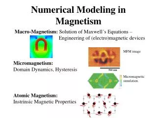
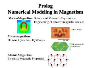
Prolog Numerical Modeling in Magnetism. Macro-Magnetism: Solution of Maxwells Equations – Engineering of (electro)magnetic devices. MFM image M icromagnetic simulation. Micromagnetism: Domain Dynamics, Hysteresis. Atomic Magnetism: Instrinsic Magnetic Properties.

E N D
PrologNumerical Modeling in Magnetism Macro-Magnetism: Solution of Maxwells Equations – Engineering of (electro)magnetic devices MFM image Micromagnetic simulation. Micromagnetism: Domain Dynamics, Hysteresis Atomic Magnetism: Instrinsic Magnetic Properties
Atomic Magnetism- Modeling Instrinsic Magnetic Properties • Band Models • Spin Polarized First Principle Methods: • restricted to simple Magnetic Structures, T=0, no dynamics, no rare earth elements ... there are attempts to overcome these restrictions • Localized Moment Models • Ising-, Heisenberg-, xy-, Standard Model of RE-Magnetism) • Exact Methods: e.g. branch and bound algorithm, transfer matrix algorithm • Monte Carlo Methods • Selfconsistent Mean Field Method
M. Rotter, Institut für physikalische Chemie, Universität Wien Atomic Magnetism- Modeling Instrinsic Magnetic Properties • Band Models • Spin Polarized First Principle Methods: • restricted to simple Magnetic Structures, T=0, no dynamics, no rare earth elements ... there are attempts to overcome these restrictions • Localized Moment Models • Ising-, Heisenberg-, xy-, Standard Model of RE-Magnetism) • Exact Methods: e.g. branch and bound algorithm, transfer matrix algorithm • Monte Carlo Methods • Selfconsistent Mean Field Method
+ + + + + + + + + + E Hamiltonian Q The Standard Model of RE Magnetism - the Crystal Field Concept 4f –charge density Martin Rotter - McPhase Course TU Dresden 2005
+ + + + + c + you can use module pointc to calculate CF parameters by the pointcharge model + + + + + + b a Example: NdCu2 Crystal Structure of RCu2 Imma (orthorhombic) ... 9 nonzero CF Parameters Martin Rotter - McPhase Course TU Dresden 2005
McPhase can • solve CF Model • Calculate Intensities and Energies • Calculate and Plot Charge Density • ... NdCu2 – Crystal Field Excitations orthorhombic, TN=6.5 K, Nd3+: J=9/2, Kramers-ion Gratz et. al., J. Phys.: Cond. Mat. 3 (1991) 9297 Martin Rotter - McPhase Course TU Dresden 2005
Module simmannfit can do this again and again for you to fit the result of the calculation to your spectrum by variation of the CF-parameters Make a Crystal Field Modelusing McPhase Module Cfield CF Hamiltonian • Example files in directory /mcphas/examples/ndcu2b_new/cf • Edit file Bkq.parameter and enter CF parameters Blm • Start module cfield - type: cfield –r -B • View output file cfield.out: CF - energies, eigenstates, transition-matrixelements and corresponding neutron intensities • Use module convolute to convolute energy vs intensity results with spectrometer resolution function Martin Rotter - McPhase Course TU Dresden 2005
Use module cfield to calculate magnetization type: cfield –m Magnetism would be boring without a magnetic field Hamiltonian Martin Rotter - McPhase Course TU Dresden 2005
Specific Heat Use module cpcalc to calculate specific heat type: cpcalc 5 30 1 Tmin=5 Tmax=30 dT=1 Martin Rotter - McPhase Course TU Dresden 2005
T=100 K T=40 K T=10 K Use modules chrgplot+javaview to plot 4f charge density Martin Rotter - McPhase Course TU Dresden 2005
Use modules pointc+chrgplot+javaview T=2K H=0 Same CEF Martin Rotter - McPhase Course TU Dresden 2005
Module mcphas Martin Rotter - McPhase Course TU Dresden 2005
Input files for module mcphas: mcphas.j (structure), mcphas.cf (single ion properties), mcphas.tst (table of initial values), mcphas.ini (H,T-range, ...) Martin Rotter - McPhase Course TU Dresden 2005
Cfield can calculate Do you really want to see the MF equations ? Martin Rotter - McPhase Course TU Dresden 2005
Bulk Properties Calculated by module mcphas Magnetization output file: mcphas.fum Martin Rotter - McPhase Course TU Dresden 2005
NdCu2 Specific Heat output file: mcphas.fum Martin Rotter - McPhase Course TU Dresden 2005
Spontaneous Magnetostriction Exchange L=0, L0 T<TC(N) „exchange-striction“ Microscopic Source of Magneostriction: Strain dependence of magnetic interactions Crystal field T T .... Symmetry decreases L0 + T>TC(N) T<TC(N) e- + Martin Rotter - McPhase Course TU Dresden 2005
Forced Magnetostriction Crystal Field Exchange Striction L0 L=0, L0 H <0 H + e- H >0 + Martin Rotter - McPhase Course TU Dresden 2005
Calculation of Magnetostriction Crystal Field Exchange mit Output file: mcphas.xyt Output file: mcphas.jj* + Martin Rotter - McPhase Course TU Dresden 2005
NdCu2 Magnetostriction Crystal Field Exchange - Striction Martin Rotter - McPhase Course TU Dresden 2005
NdCu2 Magnetic Phase Diagram F1 F3 c F1 b a AF1 lines=experiment output file: mcphas.xyt Use module phased or displaycontour for color plot of phasediagram Martin Rotter - McPhase Course TU Dresden 2005
output file: mcphas.hkl Martin Rotter - McPhase Course TU Dresden 2005
Dispersive Magnetic Excitations 153 MF - Zeeman Ansatz T=1.3 K Martin Rotter - McPhase Course TU Dresden 2005
... Spinwaves (Magnons) 153 T=1.3 K Bohn et. al. PRB 22 (1980) 5447 Martin Rotter - McPhase Course TU Dresden 2005
Spinwaves (Magnons) 153 a T=1.3 K Bohn et. al. PRB 22 (1980) 5447 Martin Rotter - McPhase Course TU Dresden 2005
MF-RPA Module Mcdisp – Calculate Magnetic Excitation Energies and the Neutron Scattering Cross Section Martin Rotter - McPhase Course TU Dresden 2005
Module Mcdisp – a novel fast algorithm for magnetic excitations – Rotter 2005 Transformation: Martin Rotter - McPhase Course TU Dresden 2005
with definition: (1) all other components of Ψ are zero with definition: Generalized eigenvalue problem (analogue to dynmical matrix in the case of phonons!!) Solution gives eigenvalues and eigenvectors Martin Rotter - McPhase Course TU Dresden 2005
may then be inverted to give the following expression for Ψ back transformation... +calculation of absorptive part... using Diracs formula: Martin Rotter - McPhase Course TU Dresden 2005
McDisp - fast algorithm - Cookbook 1) 2) 3) ...setup Matrix 4) ...solve generalized EV Problem 5) Martin Rotter - McPhase Course TU Dresden 2005
F3 F1 AF1 NdCu2
Diffuse Scattering Martin Rotter - McPhase Course TU Dresden 2005
McPhase Modules Martin Rotter - McPhase Course TU Dresden 2005
Symmetry - CF Local Point Symmetry limits the number of nonzero Crystal Field Parameters (mind: local symmetry at rare earth position may be lower than lattice symmetry, i.e. The lattice may be cubic, but the local symmetry tetragonal)
Example: 2nd order CF terms for point symmetry mm2=C2v We choose here the basis of Racah instead of Stevens operators for the Crystal field, because these transform like the spherical harmonic functions Group elements G Irr. Repr. These operators form a reducable representation T2(G) of the point group Character table of mm2 Group Theory basics taken from: Elliott&Dawber Symmetry in Physics, McMillan Press, 1979 Martin Rotter - McPhase Course TU Dresden 2005
The representation T2(G) can be decomposed into irreducible Representations (i.e. „the Olm can be linear combined to another Basis so that in this basis the representation T2 bas block diagonal form with each block corresponding to a irreducible representation“) The m‘s tell, how often a representation occurs. mA1 tells, how often the unit representation occurs in the decomposition, i.e. how many different independent basis vectors span this subspace, i.e. how many independent crystal field parameters will occur. A little group theoretical trick for calculating m Cp... Number of members of class p g.... Number of group elements χ.... Character of class a... Angle of rotation i.e. We expect 2 independent 2nd order CF parameters Martin Rotter - McPhase Course TU Dresden 2005
The basis of the 2 A1 representation occuring in the decomposition of T2(G) can be found using the projection operator In order to calculate it, we have to epxlicitely write down the reducable representation T2: Jx‘=-Jx, Jy‘=-Jy Jy‘=-Jy Jx‘=-Jx B20 and B22 are nonzero. Martin Rotter - McPhase Course TU Dresden 2005
Symmetry – Bilinear Interaction Isotropic interaction (J(ij) is a scalar) Anisotropic Interaction (J(ij) is a tensor) Martin Rotter - McPhase Course TU Dresden 2005
(quasi)hexagonal types of neighbors neighbors related by symmetry must have related interaction constants J(ij) CeCu2 Structure Cu Ce M. Rotter et al., Eur. Phys. J. B 14, 29 (2000) M. Rotteret al., JMMM. 214, 281(2000) Martin Rotter - McPhase Course TU Dresden 2005
Anisotropic Interaction –Symmetry Considerations Martin Rotter - McPhase Course TU Dresden 2005
ETC... Martin Rotter - McPhase Course TU Dresden 2005
Example: bc mirror plane b 1 a 0 Martin Rotter - McPhase Course TU Dresden 2005
Symmetry – Quadrupolar Interaction Derivation similar to CF operator using representation T(G)=T2(G)xT2 (G) • Isotropic Quadrupolar Interaction • dhcp –lattice: between hexagonal sites • dhcp –lattice: between quasicubic sites
H + M + + + + + Example for quadrupolar interactions: PrCu2 + + + + + + Martin Rotter - McPhase Course TU Dresden 2005
www.mcphase.de + + + Settai et. al. JPSJ 67 (1998) 636 + + + Ferroquadrupolarer (Cij>0) Austausch (durch CF-Phonon WW) PrCu2 GMS + + + + + + Settai et. al. JPSJ 67 (1998) 636 Martin Rotter - McPhase Course TU Dresden 2005
Ferroquadrupolar (Cij>0) Interaction PrCu2 Settai et. al. JPSJ 67 (1998) 636 • The Model describes well: • the quadrupolar phasen diagram • the magnetisation • the magnetostriction • die temperature dependence of elastic constants Whats about the Dynamics ? Martin Rotter - McPhase Course TU Dresden 2005
+ + + + + + + + + + E Crystal field +Antiferroquadrupolar (C<0) Interaction Q Orbital Excitations (Orbitonen) 4f – charge density Martin Rotter - McPhase Course TU Dresden 2005
+ + + + + + Ferroquadrupolar (Cij>0) Interaction (via CF-Phonon coupling) PrCu2 + + + + + + Settai et. al. JPSJ 67 (1998) 636 Martin Rotter - McPhase Course TU Dresden 2005
PrCu2 Orbital Modes T=5 K, H=0 T Experiment MF-RPA Model Г 2.5 Energy (meV) ? 0 1 00L 2 McPhase: www.mcphase.de Rotter, JMMM 272-276 (2003) 481 Kawarazaki et. al., J. Phys. Cond. Mat. 7 (1995) 4051 Martin Rotter - McPhase Course TU Dresden 2005
NdCu2 NdCu2 Magnetic Excitations Rotter et. al., Europ. Phys. J. B 14 (2000) 29 Könnte nicht auch die Austauschwechselwirkung zu der beobachteten Dispersion führen ? PrCu2 Nur Quadrupolaustausch Г [Interpretation von Kawarazaki et. al., J. Phys. Cond. Mat. 7 (1995) 4051] 2.5 Energy (meV) 0 1 00L 2 Martin Rotter - McPhase Course TU Dresden 2005