Download

1 / 48
480 likes | 757 Views
The Joy of Queueing Part B Dr. Mark P. Van Oyen A mixture of queueing basics, analogies, and operations management principles. Filename: 574 queue-lec-B.ppt. Waiting Line Analysis. Assists managers in determining: Likelihood a customer will have to wait (Prob of nonempty sys)

E N D
The Joy of Queueing Part B Dr. Mark P. Van Oyen A mixture of queueing basics, analogies, and operations management principles. Filename: 574queue-lec-B.ppt
Waiting Line Analysis • Assists managers in determining: • Likelihood a customer will have to wait (Prob of nonempty sys) • Average time a customer will wait (customer average –discrete) • Average number of customers waiting • (time-average – continuous) • Waiting line space needed (System design … How to address?) • Percentage of time all servers are idle (time average) • How many servers we need to employ? (System design … How to address?)
Waiting Line Analysis – cont’d Many other uses and thousands of models and formulas exist – but let us begin with the most fundamental model of queueing theory: … the M/M/1 queue. The formulas will shape our intuition and give us a knowledge of how congestion behaves.
Waiting Line Terminology • Queue - a waiting line + server(s) [we will say “queue only” if we mean to exclude the server] • Number of Servers - the workers or machines that process jobs sequentially (typically one customer at a time) [as a complication that can be addressed via simulation, workers may have different speeds and different skills]
Waiting Line Terminology – cont’d • Arrival rate (l) - (arrivals per unit of time). • M/M/1 - exp(mean 1/ l) • Service rate (m) – (service completions per unit of time). • M/M/1 - exp(mean 1/ m) • Queue discipline – tend to emphasize First-come-first-served, which is the default for the M/M/1 queue
Beyond the Arrival Rate… distribution! • Analytical models tend to assumethat customer arrivals areindependentof each other and varyrandomlyover time. • In simulations, we tend to allow greater fidelity of modeling: customer classes, complex processes generating the arrivals, etc. • For the GI/GI/1 model, the times between arrivals are called interarrival times and their distribution must be specified.
Service Times • Service Time = the time it takes to serve a task (uninterrupted). • If the model allows the service period to be interrupted (e.g., preempted by a high priority customer, or the server takes a break/vacation), then we have two standard cases: • Preemptive Resume: when service resumes, the service time remaining is computed as total service time minus time already served. • Preemptive Repeat: when service resumes, the service time remaining is computed as the original total service time (thus time already served is wasted). • M/M/1 model does not have any service interruptions
Exponential (Memoryless) Inter-arrivals • When arrivals are quite random and may come from many sources, the interarrival time is often taken to be exponential (time studies are needed to identify the actual distribution). • Exp (mean 1/ ) interarrival times imply that the number of arrivals during t units of time is a random variable with a Poisson (*t)Distribution. When *t is large, this can be approximated as a normal distribution with mean *t and standard deviation = square root(*t). • Equivalently, a Poisson(rate) arrival processes produces Exp (mean 1/ ) interarrival times
M/M/1 Model of a Gift Shop • Single Queue (channel) with a single class of customers • Infinite waiting room in the queue • The queue discipline is “first-come, first serve” • Infinite calling population (customer base). Note: With a finite population, it’s more complicated as every entity must be accounted for at all tiems. This is implicit in the assumption of the Poisson Arrival Process (exp(1/) inter-arrival times). • Single, always-available server (that’s the 1 in M/M/1) • exp(mean 1/ m) service times • only one service phase
M/M/1 Model of a Gift Shop – cont’d • Must assume something about and µ … What?
M/M/1 Model - Stability Must assume something about and µ customers are served at a faster rate than they arrive (i.e., < µ ). If >µ, …
M/M/1 Model - Stability Stability if and only if < µ If >µ, customers will continue to backup and all cannot be served. We call queues with > µ“explosive” or “unstable”. Note: In simulation, many are fooled by getting large numbers for average queue length. Is that the true average, or simply the fact that that the simulation terminated before the explosion got worse? Instability is not always easy to determine via simulation!
Queueing Variables O.M. Terms • For a GI/GI/1 system, • = system Throughput (jobs/hour) (which may be thought of as the average release rate) • µ = average capacity (jobs/hour), which is a maximum potential throughput rate.
Definitions–cont’d • r =server utilization (long run fraction of time server is busy) • P0 = probability of empty system (arrival does not wait) = 1 - r • WIP = L = average number of customers in the system (Work In Process) • Cycle Time (flowtime) = • CT = W = average cust. waiting time (queue + service)
Key Relationships of Queueing • From the perspective of an arriving customer. • Say customer number 3 is the one we want to watch: Arrival time Service time Wait in queue Cycle time (CT)
Key Relationships of Queueing • System perspective on WIP vs time: Arrival time of job 3, the “watched” customer Service time of job 3 4 3 2 1 5 1 2 3 4 5 Cycle time (CT)
Key Relationships of Queuing-cont’d • Watching the Server: • 1. Complete current job • 2. Idle if no customers present • 3. Take next customer • according to • queue discipline • = arrival event • = departure Utilization = fraction of time busy (U orr) busy busy busy idle
M/M/1 Queueing Formulae Summary server utilization = ? • The probability (P0) that no customers are in the queueing system (either in the queue or being served) • = (1 -r) = 1- /µ r = /µ = fraction of time server is busy • The average number of customers (L) in the queueing system (being serviced and in line) is • WIP = L = r / (1 - r)
M/M/1 Queueing Formulae • The average time a customer spends in the total queueing system - i.e. waiting and being served (W) CT = W = 1/(µ - ) • The average time a customer spends waiting in the queue to be served (Wq). = r /(µ - ) • U = r = The probability that the server is busy (i.e. the probability that the customer has to wait). U is the “utilization factor”
Queueing Example: M/M/1 • Jim Bream, the server, pulls stock from his warehouse shelves to fill customer orders. • Arrival time = time a customer joins checkout line, knowing what they want (not entry through doorway)
Queueing Example: M/M/1 –cont’d • The times between arrivals (called interarrival times) are exponentially distributed with arrival rate 20. Implications: • Customer orders arrive at a mean arrival rate of 20 per hour. • The number of arrivals in t hours is Poisson distributed with mean 20*t. • The service time to pull an item for any order is exponentially distributed with a mean of 2 min. (or 2/60 of an hour)
Queueing Example • Service Rate from service time distribution • Question • What is Jim’s mean service rate per hour? Answer Since Jim can process an order in an average time of 2 minutes (= 2/60 hr.), then the mean service rate, µ, is µ = 1/(mean service time), or 60/2 = 30 orders/hr.
Queueing Example • Server Utilization Factor • Question • What percentage of the time is busy Jim processing orders (as opposed to being idle)? Answer The percentage of time Jim is processing orders is equivalent to the utilization factor, r = /. Thus, the percentage of time he is processing orders is: r = / = 20/30 = 2/3 or 66.67% of the time
Queueing Example • Average Time in the System • Question • What is the average time a customer must wait from the time they join the checkout line until Jim fulfills the order (i.e. cycle time or waiting time)?
Queueing Example • Average Time in the System • Answer • With = 20 per hour and = 30 per hour, the average time an order waits in the system is: CT = W = 1/(µ - ) • = 1/(30 - 20) • = 1/10 hour or 6 minutes
Queueing Example • Average Time in the Queue (but not in service): • Question • What is the average time a customer must wait from the time they join the checkout line until Jim begins to take their order (i.e. waiting time in queue)?
Queueing Example – cont’d • Answer • With = 20 per hour and = 30 per hour, average wait time in queue is: CTq = Wq = r /(µ - ) = (2/3) * 1/(30 - 20) • = 2/30 hour or 4 minutes • Check: W = Wq + 1/ µ = 4 + 2 = 6 minutes.
Queueing Example • Average (Mean) Length of Queue • Question • What is the average number of customers waiting in line to be processed? • Answer • Try to reason it out based on the fact that there are 4 minutes of waiting time in queue prior to service. During this time, services of prior customers are occurring.
Queueing Example • Average (Mean) Length of Queue • Answer • The average number of orders waiting in the system (queue + server) is: • WIP = L = r / (1 - r) = (2/3) / (1-2/3) • = (2/3) / (1/3) • = 2 orders • This is a little surprising if you think deeply, but it is a result of memoryless property of exponential service times. The customer currently in service still seems a mean of 2 minutes (despite the “age” of the service already completed) and of course, the person in line averages 2 minutes.
Basic M/M/1 Queueing Takeaway • How does congestion (e.g., WIP) grow as the utilization of a server goes to 100%? • What if the system had multiple identical servers? (same answer, curve grows more slowly)
Little’s Law • LAW: For any “stable” queueing system (even a network of queues) • L = * W (queueing notation), that is, • WIP = TH * CT (production systems notation), • The same relationship holds if we count only the customers and time actually waiting in queue, but not being served: • Lq = * Wq • WIPq = TH * CTq
Little’s Law Example: Gas Tanks • Given: • An automotive assembly plant produces 300,000 cars per year • The length of the assembly line from the first task to the last is 1.5 miles • Gas tanks are regularly sent in batches to the plant, stored in inventory, and then used in the assembly operation. On average, the time from gas tank arrival at the plant to the completion of the finished car is 3.5 days. • How much gas tank WIP (raw material or in production) does the plant carry?
Little’s Law Example: Gas Tanks • WIP = TH * CT • (1) TH = 300,000 tanks/year • (3) CT = 3.5 days * (1 year/ 365 days) = .0096 years • WIP = 300,000 tanks/year * .0096 years • = 2,877 tanks • This is a lot, but we are producing 822 cars/day on average.
Little’s Law Example: Cash Flow • Given: • A firm carries an average annual finished goods inventory (FGI) worth $1 Billion. • Average annual sales is currently $4 Billion. • We focus on cash flow rather than product flow. • What is the average cycle time of a dollar that is put into FGI? Note: this is an aggregate model for a typical product.
Little’s Law Example: Cash Flow • Given: • WIP = $1 Billion. • TH = $4 Billion. • What is the average cycle time of a dollar that is put into FGI? WIP = TH * CT 1 B. = 4 B. * CT so the CT = WIP / TH = 1/4 year CT = 3 mo's on average that our dollar spends sitting in inventory.
Capacity Utilization vs. Customer Waiting in Services • Cost or inconvenience of waiting is usually measured by • waiting time • Blocked customers (lack of waiting space – get “busy signal”) • Customer reneging or abandonment (call center) • Fraction cust. served within X minutes • Result: • Higher utilization of service facilities • Is gained at price of customer waiting
Queuing Models and Capacity Planning • Have capacity – service level tradeoff • Goal of queueing system global optimization is: minimize total costs of • service capacity • + • waiting • What does a curve of total cost versus capacity to serve look like?
$ MIN COST LEVEL OF SERVICE Total Cost Cost of providing service Cost of customer waiting Service Level Analysis of Costs in Congested Systems High utilization,r Low utilization,r
What About Variability? • In an M/M/1 queueing model such as we have studied, the amount of variability has been fixed. I.e., regardless of the and we pick, the variability is constant (coefficient of variation (c.v.) = (std. dev. / mean ) = 1.0). In general 0 < c.v. < • The amount of variability is captured in • The interarrival distribution: c.v. = CG • The service time distribution: c.v. = CX • How does increasing variability impact the system performance?
What About Variability? M/G/1 Model • Most common application: M/G/1 • The interarrival distribution is EXPONENTIAL, c.v. = CG =1 and the arrival process is called a Poisson Process. • The service time distribution has mean 1/ , but the distribution has more or less variability: 0 < CX <
What About Variability? M/G/1 Model-cont’d • Result: Wait in queue only = ½ (1 + CX2) Wq , • Where in the M/M/1 model we defined Wq = r /(µ - ) • What does a curve of waiting time in queue versus service time variability look like?
M/G/1 Model has congestion roughly proportional to the square of std. dev. of service/process time Utilization is constant= 0.90. Taken from queue-approx.xls
Variability Principles • If, in addition, we increase the variability in the interarrival distribution: CG > 1, then we also get an increase in Queue length and waiting time (WIP and CT) that is roughly proportional to the square of the standard deviation of the interarrival time distribution. (This is from the G/G/1 model, which can only be approximated).
Role of Simulation • As we depart from exponential distributions, analysis becomes more difficult and simulation is needed in many cases • Simulation also provides the ability to model systems with • greater fidelity to the current reality • Or greater complexity IN CONTRAST, mathematical analysis is well-suited to fundamental design/evaluation and the extraction of general principles. • In Operations, simulation is often used as a research tool to perform sensitivity analysis (e.g., showing if the insights remain valid when variability departs from the CV of 1 constrained by the exponential distribution)
Variability Principles – cont’d • End result: congestion is roughly proportional to the variances of the system – interarrival and process (service) time. (i.e. proportional to standard deviations SQUARED). • Variability reduction is REALLY IMPORTANT. Cutting process time by 50% to /2 can result in a CT reduction to as low as CT/4 – even without any reduction in total, mean processing time.