Enhancing Consumer Theory through Inter-temporal Choice and Uncertainty
440 likes | 569 Views
Explore extensions to consumer theory, inter-temporal choice, and revealed preferences, diving into how consumers make satisfying choices, handle uncertainty, and spread consumption over time. Investigate the impact of interest rates, investment strategies, and decision-making under uncertainty.

Enhancing Consumer Theory through Inter-temporal Choice and Uncertainty
E N D
Presentation Transcript
Extensions to Consumer theory Inter-temporal choice Uncertainty Revealed preferences
Extensions to Consumer theory • We now know how a consumer chooses the most satisfying bundle out of the ones it can afford • From observing changes in choice that follow changes in price, we can derive the demand function. • But how useful (and realistic) is this theory? • We assumed that agents have no savings... • Does the theory still stand under uncertainty ? • We assume that stable preferences just “exist”.
Extensions to Consumer theory Inter-temporal choice Uncertainty Revealed preferences
Inter-temporal choice • The typical agents spreads his consumption over several periods of time: immediate consumption, savings, borrowing, etc. • Consume today / consume tomorrow • Current preferences between goods are convex. • Seems this is also the case for inter-temporal choices • We need to define : • Inter-temporal preferences • Inter-temporal budget constraint
Inter-temporal preferences • Preference for current consumption • A unit of consumption today is “worth” more than a unit of consumption tomorrow • I’d rather receive 100 € today than 100 € next week ! • If I give up some current consumption , I expect to receive a return (r)in compensation. • There must exist a value of (r), a psychological interest rate, for which I am indifferent between current and future consumption • Would you rather receive 100 € today or 101 € next week ? What about 120 € ?
Inter-temporal preferences • The inter-temporal indifference curve • Strictly convex et decreasing • Corresponds to an inter-temporal utility function U(C1,C2) future consumption(c2) current consumption (c1)
Inter-temporal preferences Imagine you are at A: Low current, high future consumption In order to increase your current consumption, you are willing to reduce your future consumption quite a lot future consumption(c2) A current consumption (c1)
Inter-temporal preferences At B, you are willing to give up less future consumption than at A for the same amount of extra current consumption ra > rb You are more patient! future consumption(c2) A B current consumption (c1)
Inter-temporal preferences If c1 is low : (r) is high, you are impatient If c1 is high : (r) is low, you are patient (1+r) : The MRS is a measure of patience future consumption(c2) A B current consumption (c1)
Inter-temporal budget constraint • Let’s see what happens if your savings earn interest over time. • A sum Mtinvested in t is worth Mt+1=Mt×(1+i)after 1 year • 01/08 : I invest 100 € • 12/08 : I will receive 100 × (1+i) € • If i = 0,05 (5%); Mt+1=100 × (1,05) =105 € • A invested sum Mt+1 was worth Mt=Mt+1(1+i) a year earlier • 12/08 : I receive 525 € • 01/08 : I invested 525 (1+i) € • If i = 0,05 (5%); Mt = 525(1,05)= 500 €
Inter-temporal budget constraint • Simplification: invariable price p1 = p2 = 1 • Explicit interest rate: i • Consumption : c • Budget : b • Two periods : 1 and 2
Inter-temporal budget constraint • In general, one can write: c2 = b2 + (1+i)×(b1 – c1) If (b1 – c1) > 0 lender If (b1 – c1) < 0 borrower If (b1 – c1) = 0 neither
Inter-temporal budget constraint • The budget constraint equalises the total inter-temporal budget B with the total inter-temporal consumption C : B = C • Note: Again, all the budget is spent !! Just not in the same period • There are 2 ways of expressing this budget constraint
Inter-temporal budget constraint Generic budget constraint Current value budget constraint Future value budget constraint
Inter-temporal budget constraint future consumption(c2) current consumption (c1)
C Inter-temporal budget constraint future consumption(c2) Maximum savings strategy B No borrowing / No lending Maximum borrowing strategy A current consumption (c1)
C Inter-temporal budget constraint Effect of an increase of interest rates on the inter-temporal budget constraint future consumption(c2) B A current consumption (c1)
C E Inter-temporal choice Inter-temporal choice of a lender future consumption(c2) At E: B MRS = slope of the budget constraint A current consumption (c1)
C E Inter-temporal choice Inter-temporal choice of a borrower future consumption(c2) At E we still have r=i B A current consumption (c1)
Extensions to Consumer theory Inter-temporal choice Uncertainty Revealed preferences
Uncertainty • How do we calculate the utility of an agent when there is uncertainty about which bundle will be consumed? • Example: You’re trying to decide if you want to buy a raffle ticket. What determines the potential utility of buying this ticket? • The amount of prizes and their value • The amount on tickets on sale
Uncertainty • Under uncertainty, the decision process depends on expected utility • Expected utility is simply the sum of the utilities of the different outcomes xi, weighted by the probability they will occur πi.
Good 1 Z Good 2 Uncertainty Reminder 1: preferences are assumed convex X A combination z of extreme bundles x and y is preferred to xand y x1 y1 Y x2 y2
Utility Good Uncertainty Reminder 2: Convex preferences imply a decreasing marginal utility : total utility is concave
Uncertainty • Simple illustration of uncertainty : • You have 10 units of a good and you are invited to play the following game. • A throw of heads or tail: • Probability of success or failure is 0.5 • The stake of the game is 7 units: • Outcome if you win: 17 units • Outcome if you loose: 3 units • Are you willing to play ?
Utility U(17) U(10) 0.5*U(3) + 0.5*U(17) U(3) 17 3 10 Good Uncertainty Diagram of the expected utility of the game :
Uncertainty • In this example, the expected result does not change the expected endowment of the agent. • The player starts with 10 units and the net expected gain is 0. • Even though the expected outcome is the same as the initial situation, the mere existence of the game reduces the utility of the agent. • Why is that ?
Utility U(17) U(10) U(3) Good 17 3 10 Uncertainty Risk aversion: The increase in utility following a win is smaller than the loss of utility following a loss This behavioural result is a central consequence of the hypothesis of convex preferences !!
Utility U(17) U(10) U(3) X 17 3 10 Good Uncertainty Now imagine that you do not have a choice, and you must play the game. This is a risky situation. Xrepresents the insurance premium that you are willing to pay to avoid carrying the risk
Adapting to Uncertainty/risk • Insurance: • Agents are willing to accept a smaller endowment to mitigate the presence of risk • A risky outcome, however, does not impact all agents. Insurance spreads this risk over all the agents: This is known as the mutualisation of risk. • Diversification behaviour: • Imagine you sell umbrellas: your income depends on the weather, so your future income is uncertain. • How can you make your income more certain? Sell some ice-creams on the side !! • Financial markets: • Spread the risk over many assets instead of concentrating it on a few. • You can “sell” your risk to agents that are willing to carry it, against a payment. But beware of information problems !!
Extensions to Consumer theory Inter-temporal choice Uncertainty Revealed preferences
Revealed preferences • Up until now we have assumed that preferences and indifference curves are given, and are stable • This assumption was required for the purpose of developing a theory of choice ! • But we’ve never directly observed them. How do we know we’re right? • We can reverse the theory: we work backwards from the optimal bundle and the budget constraint to get to the indifference curve. • Past choices/decisions reveal your preferences
Revealed preferences • If we have information on the bundles chosen by consumers in the past, • If we have information on the changes in prices and incomes for the duration of the period, • Then we can determine the indifference curves of the agent and verify if preferences are stable through time. • The process of revealed preferences: • Gives us information on the indifference curves • Allows us to check the realism of the assumptions behind consumer theory and the test the coherence of consumers when they make choices.
C Revealed preferences If it could be afforded, would bundle C be preferred to A ? Good 1 Without further information, we don’t know... But imagine we know of a change in prices and incomes that makes C affordable A Good 2
B C Revealed preferences B is revealed preferred to C. Therefore B≻ C Good 1 A is revealed preferred to B. Therefore A ≻B By transitivity, A is indirectly revealed preferred to C: A ≻C A Good 2
B Less desirable bundles C Revealed preferences B is revealed preferred to C. Therefore B≻ C Good 1 A is revealed preferred to B. Therefore A ≻B By transitivity, A is indirectly revealed preferred to C: A ≻C A Good 2
A B Y Z C Revealed preferences Similarly, if I see that the consumer chooses Y then Z as his income increases, I can conclude that these are revealed preferred to A. Therefore Y,Z ≻ A Good 1 Less desirable bundles Good 2
A B Y Z C Revealed preferences Good 1 Preferred bundle Less desirable bundles Good 2
A B Y Z C Revealed preferences Good 1 Preferred bundle Less desirable bundles Good 2
A B Y Z C Revealed preferences Good 1 Preferred bundle Less desirable bundles Approximation of the indfference curve Good 2
A B Y Z C Revealed preferences Good 1 Approximation of the indfference curve Good 2
A B Y Z C Revealed preferences Good 1 Approximation of the indfference curve Good 2