Optical Fibre Communication Systems

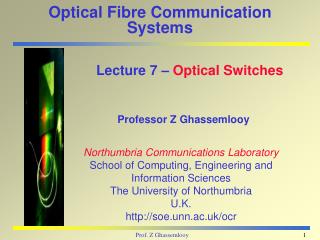
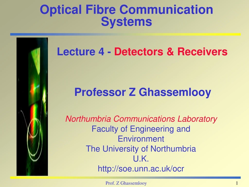
1. Optical Fibre Communication Systems Lecture 4 - Detectors & Receivers Professor Z Ghassemlooy Northumbria Communications Laboratory Faculty of Engineering and Environment The University of Northumbria U.K. http://soe.unn.ac.uk/ocr

2. Contents • Properties and Characteristics • Types of Photodiodes • PIN • APD • Receivers • Noise Sources • Performance • SNR • BER

3. Optical Transmission - Digital • The design of optical receiver is much more complicated than that of • optical transmitter because the receiver must first detect weak, distorted signals and then make decisions on what type of data was sent. • analogue receiver • But offers much higher quality than analogue receiver.

4. Optical signal (photons – hf) To recover the information signal Photo- detection Amplification (Pre/post) Filtering Signal Processing Limiting the bandwidth, thus reducing the noise power Converting optical signal into an electrical signal Information signal Optical Receiver – Block Diagram

5. Photodetection - Definition • It converts the optical energy into an electrical current that is then processed by electronics to recover the information. Detection Techniques • Thermal Effects • Wave Interaction Effects • Photon Effects

6. I Forward-biased “Photovoltic” operation Dark current V Po Short-circuit “photoconductive” operation Reverse-biased  “photoconductive” operation Photodiode - Characteristics An electronics device, whose vi-characteristics is sensitive to the intensity of an incident light wave. • Small dark current due to: • leakage • thermal excitation • Quantum efficiency (electrons/photons) • Responsivity • Insensitive to temperature variation

7. Photodetector - Types • The most commonly used photodetectors in optical communications are: • Positive-Intrinsic-Negative (PIN)  • No internal gain • Low bias voltage [10-50 V @ = 850 nm, 5-15 V @ = 1300 –1550 nm] • Highly linear • Low dark current • Most widely used • Avalanche Photo-Detector (APD) • Internal gain (increased sensitivity) • Best for high speed and highly sensitive receivers • Strong temperature dependence • High bias voltage[250 V @  = 850 nm, 20-30 V @ = 1300 –1550 nm] • Costly

8. Photons Depletion region I n p Io n p hole electron I hole electron Output RL (load resistor) Bias voltage Photodiode (PIN) - Structure • No carriers in the I region • No current flow • Reverse-biased • Photons generated electron-hole pair • Photocurrent flow through the diode and in the external circuitry The power level at a distance x into the material is: Where  is the photon absorption coefficient

9. Photodiode (PIN) - Structure Depletion region width The capacitance of the depletion layer Cj (F) is:

10. Photodetector - Reponsivity PIN: APD: R = Io/Po A/W RAPD = G R Io = Photocurrent; Po = Incident (detected) optical power G = APD gain;  = Quantum efficiency = average number of electron-hole pairs emitted re / average number of incident photons rp Note: rp = Po/hf and re = Io/q l = length of the photoactive region Io = qPo/hf Thus normally  is very low, therefore = 0. So  = 99% ~ 1

11. Photodetector - Responsivity • Silicon (Si) • Least expensive • Germanium (Ge) • “Classic” detector • Indium gallium arsenide (InGaAs) • Highest speed G Keiser , 2000

12. Contact leads Amplifier Photodiode Rs L Io Cj Rj RL Ramp Camp Output L = Large, (i.e o/c) Rs= Small, (i.e s/c) Photodetector - Equivalent Circuit CT = Cj +Camp RT = Rj ||RL || Ramp The transfer function is given by:

13. Photodetector - Equivalent Circuit The detector behaves approximately like a first order RC low-pas filter with a bandwidth of:

14. Photodiode Pulse Responses Fast response time  High bandwidth • At low bias levels rise and fall times are different. Since photo collection time becomes significant contributor to the rise time. G Keiser , 2000

15. Small area photodiode Small area photodiode Large area photodiode Due to carrier generated in w Due to diffusion of carrier from the edge of w Photodiode Pulse Responses w = depletion layer s = absorption coefficient G Keiser , 2000

16. Parameters Si PIN APD Ge PIN APD InGaAS PIN APD Wavelength range Peak (nm) 400-1100 900 830 800-1800 1550 1300 900-1700 1300 1300 (1550) (1550) Responsivity (A/W) 0.35-0.55 50-120 0.5-0.65 2.5-25 0.5-0.7 - Quantum Efficiency (%) 65-90 77 50-55 55-75 60-70 60-70 Bias voltage (-V) 45-100 220 6-10 20-35 5 <30 Dark current (nA) 1-10 0.1-1 50-500 10-500 - 1-5 Rise time (ns) 0.5-1 0.1-2 0.1-0.5 0.5-0.8 0.06-0.5 0.1-0.5 Capacitance (pF) 1.2-3 1.3-2 2-5 2-5 0.5-2 0.1-0.5 Photodetetor – Typical Characteristics Source: R. J. Hoss

17. Detector Pr Amplifier Po Power loss Minimum Received Power • Is a measure of receiver sensitivity defined for a specific: • Signal-to-noise ratio (SNR), • Bit error Rate (BER), • Bandwidth (bit rate), at the receiver output. MRP = Minimum Detected Power (MDP) – Coupling Loss

18. -20 SNR (dB) 50 30 10 0 -30 -40 MRP (-dBm) -50  =1300 -60 -70 1 2 5 10 20 50 100 200 500 1000 Bandwidth (MHz) MRP Vs. Bandwidth

19. Selection Criteria and Task Optical • Optical Sensitivity for a given BER and SNR • Operating wavelength • Dynamic range • Simplicity • Reliability and stability Electrical • Data rate • Bit error rate (digital) • Maximum Bandwidth (analogue) • Signal-to-noise ratio (analogue) Task: • To extract the optical signal (low level) from various noise disturbances • To reconstruct the original information correctly

20. Receivers: Basics • The most important and complex section of an optical fibre system • It sensitivity is design dependent, particularly the first stage or front-end • Main source of major noise sources: • Shot noise current • Thermal noise: Due to biasing/amplifier input impedance • Amplifier noise: • Current • Voltage • Transimpedance noise

21. Receiver - Bandwidth A range of frequencies that can be defined in terms of: • Spectral profile of a signal • Response of filter networks • Equivalent bandwidth: Defines the amount of noise in a system Types of Bandwidth • Ideal • Baseband • Passband • Intermediate-Channel • Transmission • Noise

22. Low-pass filter Band-pass filter 0 dB -3 Higher order filter Ideal Frequency Bbp Blp Ideal, Low-pass and Band-pass Filters

23. 0 NEB -3 dB B3dB B Filter response Noise Equivalent Bandwidth (NEB) B Defines as the ideal bandwidth describing the point where: Area under the response cure = Area under the noise curve.

24. P(t) m(t) Optical drive circuit Light source Photodiode Fibre ip(t) Amplifier Photocurrent Signal current io(t) Average photocurrent (DC current) Io Photocurrent = + Optical System

25. Optical Receiver - Model The received digital pulse stream incident at the photodetector is given by:

26. Optical Receiver - contd. For m(t) = sin t The mean square signal current is For a digital signal The mean square signal current is

27. Optical System - Noise • Is a random process, which can’t be described as an explicit function of time • In the time domain – Can be characterized in probabilistic terms as: • Mean - correspond to the signal that we are interested to recover • Variance (standard deviation) - represents the noise power at the detector’s output • Can also be characterized in terms of the Root Mean Square (RMS) value Time average

28. Optical System - Noise • The electric current in a photodetector circuit is composed of a superposition of the electrical pulses associated with each photoelectron • The variation of this current is called shot noise

29. Optical System - Noise Sources • At the receiver: • Additive • Signal dependent • Modal noise Due to interaction of (constructive & destructive) multiple coherent modes, resulting in intensity modulation. • Photodetector Noise  • Preamplifier (receiver) Noise  • Distortion due to Non-linearity • Crosstalk and Reflection in the Couplers

30. Noise Budget Noise terms • ηLD - Laser diode slope efficiency in mW/mA, • ηFO = 10-0.1(dB Loss) - Total attenuation of the fibre optic media, • ηPD = R - Photodiode responsivity in mA/mW, and • ηRX - Preamplifier gain in V/A. • Not that, all of the coupling coefficients and scale factors are lumped into these four constants, and their frequency dependence has been neglected, which is a major simplification. • With a few exceptions, all of the noise sources are assumed to be Gaussian Digital decision circuit

31. Noise Budget • With a few exceptions, all of the noise sources are assumed to be Gaussian. • The sum of two or more Gaussian PDFs yields a third Gaussian PDF, whose variance will equal the sum of the variance of the summed PDFs. • For the simple BER model adopted here, we can need to know the noise terms for the “1” and “0” levels

32. Noise -Source Noise - contd. • Light source driver • have a given IRMS noise current over a given bandwidth • Is converted to an optical noise by the light source • Defined as the equivalent optical noise variance at the PD input: For lossless fibre (ideal case), we have In terms of actual power IRMS = I = RPo A/Hz A/Hz A Rx bandwidth

33. Noise -Source Noise - contd. • LED: Due to: • In-coherent intensity fluctuation • Beat frequencies between modes • LD: Due to: • Non-linearities • Quantum noise: In the photon generation • Mode hopping: Within the cavity • Reflection from the fibre back into the cavity, which reduces coherence • Difficult to measure, to isolate and to quantify • Most problematic with multimode LD and multimode fibre • The variance due to the relative intensity noise (RIN) is given as: A2 = W

34. Noise Currents • Let noise current be defined as: inoise(t) = i(t) - IDC (Amps) IDC = Photocurrent Io Noise current from random current pulses is termed as shot-noise. • Shot-noise: • Quantum • Dark current

35. Quantum Shot Noise The photons arrive randomly in a packet form, with no two packets containing the same amount of photons. Random generation of electron-hole pair, thus current. Variation of the total current generated, about an average value. This variation is best known as QUANTUM SHOT NOISE.

36. Quantum Shot Noise • The average number of electron-holes pairs per bits is: Where  the time period. The probability of detecting n photons in a time period  is follows the Poisson Distribution: Incoherent light Y Semenova, DIT, Ireland Coherent light

37. Quantum Shot Noise The rate of electron-hole pairs generated by incident photons is: With an ideal receiver with no noise we have: Note that, the minimum pulse energy of the quantum limit is:

38. Shot Noise - PIN • The mean square quantum shot noise current on Io • The mean square dark current noise (also classified as shot noise) Where Id= surface leakage current, and B is the electrical bandwidth of the system Q is the electron charge. Total shot noise current ITs = Dark current + Photocurrent The total mean square shot noise

39. Power spectrum I2o ITs2 Shot noise Frequency 0 B Modulation bandwidth Noise Power Spectrum

40. Bias voltage hf Vo Av RL Vi Shot Noise - APD • The mean square photocurrent noise where F = The noise figure = Gx for 0<x<1 G = The optical gain

41. Noise Currents - contd. Thermal Noise RL = Total load seen at the input of the preamplifier K = Boltzmann’s constant = 1.38x10-23 J/K T = Temperature in degree Kelvin = Co + 273 Total Noise PIN APD

42. Electrical Amplifier Noise Amplifier typeBJT JEFT - Voltage Noise - Current Noise Total amplifier noise

43. “Off-the-shelf” Receiver Example

44. Receiver Signal-to-Noise Ratio (SNR) There is no universal definition of SNR. Here, we adopt a convention for both electrical and optical SNRs. Note: Ne = (e)2 Note: V  Poand No = v Po One fundamental design limit would be for the noise at the “0” level to be negligible (i.e., 0= 0 compared to the noise at the “1” level. This would be for an ideal noiseless detector and is called the “shot noise limit”. This a ultimate goal or fundamental limit that is used as a base to compare real systems. So the Q-factor

45. io iT iA Receiver Signal-to-Noise Ratio (SNR) hf • PIN • APD Note: SNR cannot be improved be amplification

46. SNR - Quantum Limit The mean square quantum shot noise current on Io Shot noise Poisson

47. Av Vo hf Vi CT RL • RC limited bandwidth Type of Receivers - Low Impedance Voltage Amplifier • Simple • Low sensitivity • Limited dynamic range • It is prone to overload and saturation RL= Rdetector ||Ramp. Ramp= High

48. Equaliser Av Vo hf Vi CT RL Type of Receivers - High Impedance Voltage Amplifier with Equaliser • High sensitivity • Low dynamic range • Rdetectoris large to reduce the effect of thermal noise • Detector out put is integrated over a long time constant, and is restored by differentiation

49. RF Bandwidth Av hf Vo Vi CT RL Type of Receivers - Transimpedance Feedback Amplifier • The most widely used  • Wide bandwidth • High dynamic range • No equalisation • Greater dynamic range (same gain at all frequencies) • Slightly higher noise figure than HIVA

50. -A Vi Vi Transimpedance Feedback Amplifier Where is the noise power spectral density, and RT = RL||RF