Download
1 / 51
800 likes | 2.53k Views
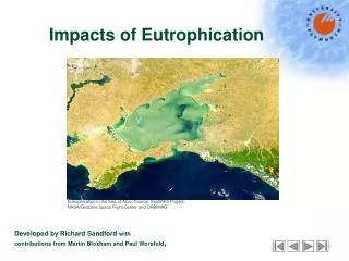
5. EUTROPHICATION OF LAKES. Like winds and sunsets, wild things were taken far granted until progress began to do away with them. - Aldo Leopold, A Sand County Almanac. 5.1. INTRODUCTION.

E N D
5. EUTROPHICATION OF LAKES Like winds and sunsets, wild things were taken far granted until progress began to do away with them. - Aldo Leopold, A Sand County Almanac
5.1. INTRODUCTION • Eutrophication: excessive rate of addition of nutrients (usually: anthropogenic activities and the addition of phosphorus and nitrogen to natural waters). • Nutrient additions result in the excessive growth of plants including phytoplankton (free-floating algae), periphyton (attached or benthic algae), and macrophytes (rooted, vascular aquatic plants). • Natural process taking place over geologic time that is greatly accelerated by human activities. For example, due to soil erosion and biological production, lakes normally fill with sediments over thousands of years; but eventually the process is accelerated to decades.
Undesirable effects of water quality: • Excessive plant growth (green color, decreased transparency, excessive weeds). • Hypolimnetic loss of dissolved oxygen (anoxic conditions). • Loss of species diversity (loss of fishery). • Taste and odor problems. • Not all eutrophic lakes will exhibit all of these water quality problems, but they are likely to have one or more of them. • Eutrophication is excessive rate of addition of nutrients. • Water quality may become so degraded that the lake's original uses are lost, being no longer be swimmable or fishable.
Figure 5.1. Schematic of lake eutrophication and nutrient recycle. Thermal stratification causes a high concentra-tion of oxygen in near-surface waters, but the dissolved oxygen cannot mix vertically, and deep water eventually becomes anoxic. Anoxic conditions in the bottom waters and sediments cause anaerobic decomposition and the release of nutrients (phos-phate, ammonia, dissolved iron).
The degree of eutrophication is a continuum. It is referred to as the “trophic status” of the water body: • Oligotrophic (undernourished – biological production is limited by nutrient additions); • Mesotrophic; • Eutrophic (well-nourished). • Phosphate is often the limiting nutrient for algal growth, and point sources are reduced by precipitation of phosphate in wastewater with iron chloride or iron sulfate. • Nonpoint sources are caused by agricultural runoff, stormwater runoff, or combined-sewer overflow. Both particulate and dissolved forms of nutrient additions are important. • Bioavailability of nutrients debate as to the relative contribution of particulate and adsorbed nutrients to the eutrophication of lakes.
5.2. STOICHIOMETRY • Primary production in natural waters is the photosynthetic process whereby carbon dioxide and nutrients are converted to plant protoplasm. • Respiration is the reverse process in which protoplasm undergoes endogenous decay and/or lysis and oxidation: • Algal protoplasm: C106H263O110N16P1 • Algal respiration occurs during both dark and daylight hours, but photosynthetic primary production can occur only in the presence of sunlight. • Algae settle and decay, and the nutrients recycle from the sediment back to the overlying water.
Figure 5.2. Regulation of the chemical composition of natural waters by algae.
Stoichiometry helps to determine the ratios of elements assimilated during primary production for mathematical modeling. It also helps us to understand the regulation of the chemical composition of natural waters. • The molar ratio of nitrogen to phosphorus is 16:1, as indicated by the stoichiometric equations. Algae assimilate nutrients in these ratios and when algal cells lysis and decompose (Figure 5.3), they release the N and P in the same molar ratios, thus regulating, to some extent, the chemical composition of natural waters. • Martin and co-workers: relatively high concentrations of nitrate and phosphate in Antarctic seas is due to the extremely small amounts of dissolved iron in solution, which limits phytoplank-ton growth.
Figure 5.3. Ratio of nitrate to phosphate in surface ocean waters.
Example 5.1. Nutrient Assimilation Rates Based on Algal Uptake Stoichiometry Assuming the stoichiometric relationship for algal protoplasm, estimate the nutrient uptake rate for nitrate and CO2 in Lake Ontario. It was observed that 5µg per liter of phosphate was removed from the euphotic zone during the month of May in Lake Ontario. What is the rate of phytoplankton production in biomass, dry weight? Solution: Use stoichiometric ratios to convert from phosphorus to biomass.
(31 days) (18.5 μgL-1 d-1) = 573 µg L-1 algae 0.57 mg L-1 of algae grew during the month of May in Lake Ontario
5.3. PHOSPHORUS AS A LIMITING NUTRIENT • It is possible that one of many nutrients could limit algal growth. • Parsons and Takahash: the following micronutrients are impor-tant for photosynthesis. • Macronutrients: CO2 (the carbon source), phosphorus, nitrogen (ammonia or nitrate), Mg, K, Ca, and dissolved silica for diatom frustule formation. • Algae and rooted aquatic plants are photoautotrophs-they use sunlight as their energy source and CO2 for their carbon source. • The terminal electron acceptor is usually dissolved oxygen in the electron transfer of photosynthesis.
Any of these nutrients could become limiting for growth, as per Liebig's law of the minimum from the 19th century. • Liebig envisioned a saturated response growth curve for each nutrient, similar to that shown for Monod kinetics (Figure 5.4). μmax – maximum growth rate, S – substrate or nutrient concentration, Ks – half-saturation constant. • It is possible that more than one nutrient will become limiting for growth at the same time. Di Toro - evaluated the expressions for an electrical resistance analogue in parallel: and a multiplicative analogue:
Figure 5.4. Response curves of algal growth rates to limiting nutrients, light, and temperature.
Example 5.2.Limiting Nutrient Concentrations and Overall Growth Rates Estimate the resulting growth rate for diatom phytoplankton in the Great Lakes by three different methods for the following data if the maximum growth rate is 1.0 per day. - Liebig’s law of the minimum. - Electrical resistance analogy. - Multiplicative algorithm. Solution: a) Monod kinetic expressions: Liebig: the min growth rate is the appropriate choice the answer is 0.2 d-1.
b) Electrical resistance analogy: All three nutrients contribute to an overall growth rate. c) Multiplicative algorithm: The multiplicative law also includes limitation due to all three nutrients, and it result in the lowest predicted growth rate of all three methods. Experiment studies with all three nutrients in combination would be needed to confirm which model is most accurate.
5.4. MASS BALANCE ON TOTAL PHOSPHORUS IN LAKES • A simple mass balance can be developed on the limiting nutrient in a lake, e.g., total phosphorus. • Here: total phosphorus – unfiltered concentration of inorganic, organic, dissolved, and particulate forms of phosphorus. • For steady flow and constant volume: lake is a completely mixed flow-through system (Pout = Plake). • The average lake concentration is equal to the concentration of total phosphorus in the outflow. V – lake volume; P – total phosphorus concentration; Qin – inflow rate; Pin – inflow total phosphorus concentration; ks – first-order sedimen-tation coefficient, Q – outflow rate.
The sedimentation coefficient is surrogate parameter for the mean settling velocity, reciprocal mean depth, and an alpha factor for the ratio of particulate phosphorus to total phosphorus α – ratio of particulate P to total P, vs – mean particle settling velocity, H – mean depth of the lake • Under conditions of steady-state the eq`n can be simplified: • If evaporation can be neglected, the inflow rate is approximately equal to the outflow rate. τ – hydraulic detention time.
Total P concentration is directly related to the total P concentra-tion in the inflow (Pin), and it is inversely related to the hydrau-lic detention time and the sedimentation rate constant (the main removal mechanism of total phosphorus from the water column). The fate of total phosphorus in lakes is determined by an impor-tant dimensionless number (ksτ). • There is a trade-off between the detention time of the lake and the sedimentation rate constant — it is the product of these two parameters that determines the ratio of total phosphorus in the lake to the inflowing total P: • The fraction of total phosphorus that is trapped or removed from the water column:
Example 5.3.Mass Balance on Total Phosphorus in Lake Lyndon B. Johnson Lake Lyndon B. Johnson is a flood control and recreational reservoir along a chain of reservoirs in central Texas along the Colorado River. It has an average hydraulic detention time of 80 days, a volume of 1.71 × 10⁸ m3, and a mean depth of 6.7 m. The ratio of particulate to total phosphorus concentration in the lake is 0.7, and the mean particle settling velocity is 0.1 m d-1. If the flow-weighted average inflow concentration of total phosphorus to Lake LBJ is 72 µg L-1, estimate the average annual total phosphorus concentration in the lake. Solution:
The answer is a total phosphorus concentration of 39 µg L-1 in the lake, 70% of which is particulate material and the remaining 30% is dissolved (most of the dissolved P is PO43- available for phytoplankton uptake). The mass flux of total P to the bottom sediment is ksPV, a flux rate equal to 69 kg d-1. A plot of the fraction of total P remaining in any lake as a function of the dimensionless number ksτ is given by Figure 5.5. The fraction of total P removed to the lake sediments is equal to 0.454 (1 - P/Pin); the mass of total phosphorus entering the lake is 152 kg d-1 and the mass outflow is 83 kg d-1 (Figure 5.6).
Figure 5.5. Fraction of total P remaining in a lake as a function of the sedimentation coefficient ks times the detention time τ
Figure 5.6. Total P mass balance for Lake Lyndon B. Johnson in central Texas
5.5. NUTRIENT LOADING CRITERIA • Clair Sawyer was one of the first investigators to consider adoption of a criterion for the classification of eutrophic lakes. • Vollenweider: not the nutrient concentration that mattered as much as the nutrient supply rate. He published "permissible" and ''dangerous" loading rates for lakes based on a log-log plot of annual phosphorus loading versus mean depth, which became widely adopted as nutrient loading criteria - classify lakes as oligotrophic, mesotrophic, and eutrophic. • Actually, both approaches to classifying the trophic status are valid and interrelated.
Dillon and Rigler modified the Vollenweider approach to account for lakes of varying hydraulic detention times and phosphorus retention (fraction removed). • improved the empirical fit of the observed lake conditions and their trophic classification; • firmly grounded the classification criteria on mass balance principles. • Now possible to determine the mean total phosphorus concentrations that defined the classification scheme (Figure 5.7). • Oligotrophic lakes: less than 10 µg L-1 total phosphorus on an annual average basis. • Eutrophic lakes: greater than 20 µg L-1 total phosphorus concentrations. • Mesotrophic lakes: intermediate with total P concentrations between 10 and 20 µg L-1.
Areal nutrient (phosphorus) loading rate – L the mass balance: • Dividing through by the volume of the lake (V = AsurfH): νs – mean apparent settling velocity of total phosphorus. • At steady-state (dP/dt = 0) the eq`n is simplified to: • The final equation describing Figure 5.7 is: ρ – hydraulic flushing rate of the lake (1/τ).
A log-log plot of nutrient loading remaining, L(1-R)/ρ, versus mean depth (H) will have a slope of 1.0 and an intercept where H = 1 m of log P. • Lorenzen, Larsen: similar simple mass balance models for predicting total P concentration in lakes – the concepts of total P loading on an areal basis and an apparent settling velocity at steady state. • Multiplying by the mean depth H: qs – surface overflow rate for the lake (Q/Asurf)
5.6. RELATIONSHIP TO STANDING CROP • The nuisance conditions of a eutrophic lake are not only nutrient concentrations, but rather: • excessive algal blooms; • decreased transparency; • decaying algae in the sediment (consumes oxygen, ruins aquatic habitats, causes taste and odor problems). • Previous mass balance models: predict steady-state or annual average total P, but do not predict biomass or chlorophyll α (phytoplankton pigments as a measure of standing crop). • Other investigations: it is possible to correlate the summer concentration of total P to the chlorophyll concentration (Figure 5.8).
Figure 5.8. Relationship between summer levels of chlorophyll a and measured total phosphorus concentration for 143 lakes.
Phytoplankton primary use ortho-phosphate (PO4-3) measured as molybdate-reactive phosphoruse. Figure 5.8 is valid because total P is correlated with ortho-phosphorus, which is bioavailable to phytoplankton. • Other limnological measures can be correlated with chlorophyll a or trophic status of lakes. • Other indicators of eutrophic conditions: • Cyanobacteria (blue-green algae) blooms. • Loss of benthic invertebrates such as mayfly larvae (Hexagenia spp.). • Secchi disk depths less than 2.0 meters. • Loss of fishery and presence of "rough" fish. • Taste and odor problems. • Aquatic weeds in littoral zones. • Chlorophyll a concentrations greater than 10 µg L-1.
5.7. LAND USE AND BIOAVAILABILITY • Major inputs, to streams and lakes that present a difficult challenge for water quality management and control: • nonpoint source runoff, particularly from intensive agriculture; • urban stormwater runoff; • combined-sewer overflow. • Bioavailability of the nutrients becomes important when much of the runoff from nonpoint sources is in organic or particulate forms that algae cannon use directly. Also, the oxygen content of bottom waters has an effect on bioavailability. • Several empirical models for estimating nonpoint source nutrient loadings to natural waters and the net phosphorus retention of lakes. It is too simplistic to assume that all of the phosphorus that settles to the bottom sediments of a lake remains there.
When costly decisions are necessary for water quality management, it is desirable to use a more detailed and mechanistic approach to the eutrophication problem (nonlinear interactions between nutrients, plankton, and dissolved oxygen). • Limitations and assumptions: • Steady state, completely mixed assumptions. • One limiting nutrient assumption. • No recycle of nutrients from sediments. • Lack of a dissolved oxygen mass balance that triggers sediment release of nutrients under anoxic conditions.
5.5. DYNAMIC ECOSYSTEM MODELS FOR EUTROPHICATION ASSESSMENTS • Many cases: a better methodology is needed rather than a steady-state, total phosphorus model for assessing the eutrophication of lakes. • Chapra: extended the concept of the Vollenweider approach to a dynamic (time-variable) lake model for total phosphorus in the Great Lakes with sedimentation as the major loss mechanism (Figure 5.9). • At the same time (late 1970s), a variety of dynamic ecosystem models were developed by DiToro, Thomann, and O'Connor that included nitrogen, silica, and phosphorus limitation, as well as zooplankton grazing and loss terms.
Figure 5.9. Dynamic model simulation of total phosphorus in the Great Lakes by Chapra.
Figure 5.10: general schematic of a dynamic ecosystem model • Water quality includes nutrients, chlorophyll a, transparency, and dissolved oxygen. • Figure 5.11: typical flowchart for phosphorus in the Lake Erie model • Available phosphorus is commonly taken to be ortho-phosphate (PO43-) that passes a 0.45-µm membrane filter. • Unavailable particulate phosphorus is everything else that is measured in a whole water sample for total phosphorus. • More than one taxa of phytoplankton contribute to the aggregate measurement of chlorophyll a in lakes. • In northern temperate lakes, a spring bloom of diatoms (cold-water phytoplankton with silica frustules) is often followed by a summer bloom of green algae or a late summer-early fall bloom of cyanobacteria (blue-green algae). Figure 5.12 illustrates a double phytoplankton bloom in Lake Ontario.
Figure 5.10. Schematic of an aquatic ecosystem
Figure 5.11. Flowchart for phosphorus kinetics in a dynamic ecosystem model
Figure 5.12. A dynamic eutrophication model calibration for Lake Ontario with two phytoplankton species (diatoms and nondiatoms)
Blue-green algae especially can cause water quality problems because they • float (because of the gas vacuoles in the cell formed during nitrogen-fixation of some blue-green algae with heterocysts) • are associated with taste and odor problems and toxins during their decay following the bloom • difficult to control (do not need many nutrients and have very low loss rates – no sinking) • Phytoplankton taxa:
Phytoplankton must be modeled within the context of their transport regime. • Ecological niches within a lake: • Littoral – shallow water, near shore. • Pelagic – open water, deep. • Euphotic zone – light penetration to 1-10% of near-surface light. • Epilimnion – above the thermocline, well-mixed. • Hypolinmion – below the thermocline, well-mixed. • Sediment-water interface – bioturbation, diffusion of pore water, variable redox conditions. • Figure 5.13: transport regime for a large lake ecosystem. It is necessary to compartmentalize the lake into a number of compartments to account for transport and unique ecological features of each zone – six-compartment model with three surface layers (epilimnetic compartments) and three deep layers (hypolimnetic compartments).
Figure 5.13. Transport regime for a compartmentalized lake ecosystem model. Large arrows represent current flow (advection) and double; small arrows – mixing (dispersion) between compartments.
The first step in developing a dynamic ecosystem water quality model is to determine the transport regime quantitatively. This is usually accomplished by simulating momentum, heat, or mass transport of a constituent that is well known and independent of water quality. • The method of determining the correct transport regime is one of the following: • Velocity field (momentum). • Temperature distribution (heat). • Conservative tracer (chloride or total dissolved solids).
For a conservative tracer such as chloride in large 3-D lakes, for j-th compartment: Vj – volume of the j-th comp.; Cj – concentration of a conservative tracer in the j-th comp.; Qij – flowrate from the j-th to the i-th adjacent comp.; Eij – bulk dispersion coefficient between the j-th and the i-th adjacent comp.; Aij – interfacial area between the j-th and the i-th adjacent comp.; Ci – concentration of a conservative tracer in the i-th comp.; lij – half-distance (connecting distance between the middle of the two adjacent compartments). • Bulk dispersion coefficient is scale dependent as an aggregate formulation of all mixing processes (may be thought of as a bulk exchange flow going each way between compartments in Figure 5.13)
Procedures for model calibration and verification are: • Calibrate the model using field data for a conservative substance (e.g., chloride) or heat to determine Qij and Eij values. • Using the same advective flows and bulk dispersion coefficients between compartments, calibrate the model for all water quality constituents for the same set of field data to determine all other adjustable parameters and coefficients (reaction rate constants, stoichiometric coefficients, etc.). • Verify the model with an independent set of field data, keeping all transport and reaction coefficients the same. Determine the "goodness of fit" between the model results and field data. • A suitable criterion for acceptance of the model calibration and verification should be determined a priori, depending on the use of the model in research or water quality management. • A median relative error of 10 - 20%, model results/field data, is typical in water quality models.
Ecosystem models consist of a series of mass balance equations within each compartment. • The number of compartments will vary depending on the spatial extent of water quality data that is available and the resolution that is needed from the model. • Figure 5.14: a schematic of a typical ecosystem model. • nine state variables shown, but there could be more or less depending on the design of the model. • each of the nine state variables will undergo advection and dispersion as shown in the previous equation; however, fish and zooplankton would not disperse at the same rate as other water quality constituents because they are motile. • assume four limiting nutrients and a multiplicative expression here. • biomass, rather than chlorophyll a or carbon, is simulated.
Figure 5.14. Ecosystem model for eutrophication assessments. Boxes represent state variables; solid arrows are mass fluxes; and dotted lines represent external forcing functions.
Temperature affects every rate constant, increasing the rate of the reaction.
where: • These equations describe quantitatively the interactions of Figure 5.14. • Table 5.5 gives a range and a typical value for the parameters, coefficients, and rate constants used in the model.
Table 5.5. Rate Constants and Stoichiometric Coefficients for Dynamic Ecosystem Models