Download
1 / 39
390 likes | 415 Views
Explore Bayesian model selection, neurocomputational models, and model comparison methods in Dynamic Causal Modeling (DCM) for fMRI applications at a specialized course. Learn about BMS, parameter estimates, model evidence, and approximations to enhance model selection and inference techniques. Compare model families, understand DCM complexities, and delve into BMA and Bayes factors for effective model evaluation.

E N D
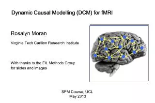
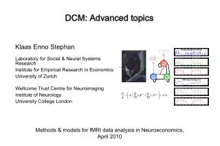
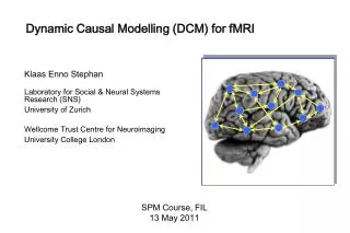
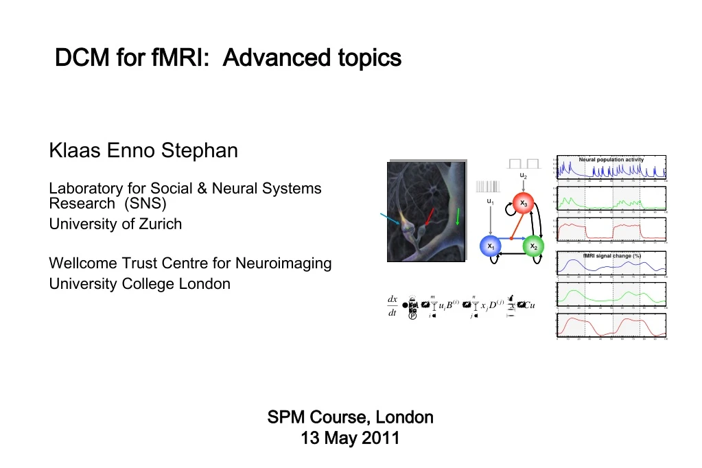
DCM for fMRI: Advanced topics Klaas Enno Stephan Laboratory for Social & Neural Systems Research (SNS) University of Zurich Wellcome Trust Centre for Neuroimaging University College London SPM Course, London 13 May 2011
Dynamic Causal Modeling (DCM) Hemodynamicforward model:neural activityBOLD Electromagnetic forward model:neural activityEEGMEG LFP Neural state equation: fMRI EEG/MEG simple neuronal model complicated forward model complicated neuronal model simple forward model inputs
Overview • Bayesian model selection (BMS) • Neurocomputational models:Embedding computational models in DCMs • Integrating tractography and DCM
definition of model space inference on model structure or inference on model parameters? inference on individual models or model space partition? inference on parameters of an optimal model or parameters of all models? optimal model structure assumed to be identical across subjects? comparison of model families using FFX or RFX BMS optimal model structure assumed to be identical across subjects? BMA yes no yes no FFX BMS RFX BMS FFX BMS RFX BMS FFX analysis of parameter estimates (e.g. BPA) RFX analysis of parameter estimates (e.g. t-test, ANOVA) Stephan et al. 2010, NeuroImage
Pitt & Miyung (2002) TICS Model comparison and selection Given competing hypotheses on structure & functional mechanisms of a system, which model is the best? Which model represents thebest balance between model fit and model complexity? For which model m does p(y|m) become maximal?
Bayesian model selection (BMS) Model evidence: Gharamani, 2004 p(y|m) y all possible datasets accounts for both accuracy and complexity of the model • Various approximations, e.g.: • negative free energy, AIC, BIC allows for inference about structure (generalisability) of the model McKay 1992, Neural Comput. Penny et al. 2004a, NeuroImage
Approximations to the model evidence in DCM Maximizing log model evidence = Maximizing model evidence Logarithm is a monotonic function Log model evidence = balance between fit and complexity No. of parameters In SPM2 & SPM5, interface offers 2 approximations: No. of data points Akaike Information Criterion: Bayesian Information Criterion: AIC and BIC only take into account the number of parameters, but not the flexibility they provide (prior variance) nor their interdependencies.
The (negative) free energy approximation • Under Gaussian assumptions about the posterior (Laplace approximation), the negative free energy F is a lower bound on the log model evidence: • F can also be written as the difference between fit and complexity:
The complexity term in F • In contrast to AIC & BIC, the complexity term of the negative free energy F accounts for parameter interdependencies. • The complexity term of F is higher • the more independent the prior parameters ( effective DFs) • the more dependent the posterior parameters • the more the posterior mean deviates from the prior mean • NB: Since SPM8, only F for is used for model selection !
Bayes factors To compare two models, we could just compare their log evidences. But: the log evidence is just some number – not very intuitive! A more intuitive interpretation of model comparisons is made possible by Bayes factors: positive value, [0;[ Kass & Raftery classification: Kass & Raftery 1995, J. Am. Stat. Assoc.
M3 attention M2 better than M1 PPC BF 2966 F = 7.995 stim V1 V5 M4 attention PPC stim V1 V5 BMS in SPM8: an example attention M1 M2 PPC PPC attention stim V1 V5 stim V1 V5 M3 M1 M4 M2 M3 better than M2 BF 12 F = 2.450 M4 better than M3 BF 23 F = 3.144 Stephan et al. 2008, NeuroImage
Fixed effects BMS at group level Group Bayes factor (GBF) for 1...K subjects: Average Bayes factor (ABF): Problems: • blind with regard to group heterogeneity • sensitive to outliers
Random effects BMS forheterogeneousgroups Dirichlet parameters = “occurrences” of models in the population Dirichlet distribution of model probabilities r Multinomial distribution of model labels m Model inversion by VariationalBayes (VB) or MCMC Measured data y Stephan et al. 2009a, NeuroImage Penny et al. 2010, PLoS Comp. Biol.
LD LD|LVF LD|RVF LD|LVF LD LD RVF stim. LD LVF stim. RVF stim. LD|RVF LVF stim. MOG MOG MOG MOG LG LG LG LG FG FG FG FG m2 m1 m2 m1 Data: Stephan et al. 2003, Science Models: Stephan et al. 2007, J. Neurosci.
m2 m1 Stephan et al. 2009a, NeuroImage
Model space partitioning: comparing model families m2 m1 m2 m1 Stephan et al. 2009, NeuroImage
Comparing model families – a second example • data from Leff et al. 2008, J. Neurosci • one driving input, one modulatory input • 26 = 64 possible modulations • 23 – 1 input patterns • 764 = 448 models • integrate out uncertainty about modulatory patterns and ask where auditory input enters Penny et al. 2010, PLoS Comput. Biol.
Bayesian Model Averaging (BMA) • abandons dependence of parameter inference on a single model • computes average of each parameter, weighted by posterior model probabilities • represents a particularly useful alternative • when none of the models (or model subspaces) considered clearly outperforms all others • when comparing groups for which the optimal model differs NB: p(m|y1..N) can be obtained by either FFX or RFX BMS Penny et al. 2010, PLoS Comput. Biol.
5 10 Number of models 4 10 3 10 2 10 1 10 0 10 2 3 4 5 6 number of nodes Log-evidence BMS for large model spaces 100 0 -100 -200 • for less constrained model spaces, search methods are needed • fast model scoring via the Savage-Dickey density ratio: Free-energy -300 -400 assuming reciprocal connections -500 -600 -600 -500 -400 -300 -200 -100 0 100 Savage-Dickey Friston et al. 2011, NeuroImage Friston & Penny 2011, NeuroImage
BMS for large model spaces Log-posterior Model posterior 100 0.9 • empirical example: comparing all 32,768 variants of a 6-region model (under the constraint of reciprocal connections) 0.8 0 0.7 0.6 -100 0.5 log-probability probability 0.4 -200 0.3 0.2 -300 0.1 -400 0 0 0.5 1 1.5 2 2.5 3 3.5 0 0.5 1 1.5 2 2.5 3 3.5 4 4 model model x 10 x 10 MAP connections (full) MAP connections (sparse) 0.8 0.8 0.6 0.6 0.4 0.4 0.2 0.2 0 0 -0.2 -0.2 -0.4 -0.4 -0.6 -0.6 0 5 10 15 20 25 30 35 0 5 10 15 20 25 30 35 Friston et al. 2011, NeuroImage
Overview • Bayesian model selection (BMS) • Neurocomputational models:Embedding computational models in DCMs • Integrating tractography and DCM
Conditioning Stimulus Target Stimulus or 1 0.8 or 0.6 CS TS Response 0.4 0 200 400 600 800 2000 ± 650 CS 1 Time (ms) CS 0.2 2 0 0 200 400 600 800 1000 Learning ofdynamic audio-visualassociations p(face) trial den Ouden et al. 2010, J. Neurosci.
1 True Bayes Vol HMM fixed 0.8 HMM learn RW 0.6 p(F) 450 0.4 440 0.2 430 RT (ms) 420 0 400 440 480 520 560 600 Trial 410 400 390 0.1 0.3 0.5 0.7 0.9 p(outcome) Explaining RTs by different learning models Reaction times Bayesian model selection: hierarchical Bayesianmodel performsbest • 5 alternative learning models: • categorical probabilities • hierarchical Bayesian learner • Rescorla-Wagner • Hidden Markov models (2 variants) den Ouden et al. 2010, J. Neurosci.
k vt-1 vt rt rt+1 ut ut+1 1 0.8 0.6 p(F) 0.4 0.2 0 400 440 480 520 560 600 Trial Hierarchical Bayesian learning model volatility probabilistic association observed events Behrens et al. 2007, Nat. Neurosci.
p < 0.05 (SVC) 0 0 -0.5 -0.5 BOLD resp. (a.u.) BOLD resp. (a.u.) -1 -1 -1.5 -1.5 -2 -2 p(F) p(H) p(F) p(H) Stimulus-independent prediction error Putamen Premotor cortex p < 0.05 (cluster-level whole- brain corrected) den Ouden et al. 2010, J. Neurosci.
Prediction error (PE) activity in the putamen PE during reinforcement learning O'Doherty et al. 2004, Science PE during incidental sensory learning den Ouden et al. 2009, Cerebral Cortex According to current learning theories (e.g., free energy principle): synaptic plasticity during learning = PE dependent changes in connectivity
Plasticity of visuo-motor connections Hierarchical Bayesian learning model • Modulation of visuo-motor connections by striatalprediction error activity • Influence of visual areas on premotor cortex: • stronger for surprising stimuli • weaker for expected stimuli PUT p= 0.017 p= 0.010 PMd PPA FFA den Ouden et al. 2010, J. Neurosci.
Prediction error in PMd: cause or effect? Model 1 Model 2 model 2 model 1 den Ouden et al. 2010, J. Neurosci.
Overview • Bayesian model selection (BMS) • Neurocomputational models:Embedding computational models in DCMs • Integrating tractography and DCM
Diffusion-weighted imaging Parker & Alexander, 2005, Phil. Trans. B
Probabilistic tractography: Kaden et al. 2007, NeuroImage • computes local fibre orientation density by spherical deconvolution of the diffusion-weighted signal • estimates the spatial probability distribution of connectivity from given seed regions • anatomical connectivity = proportion of fibre pathways originating in a specific source region that intersect a target region • If the area or volume of the source region approaches a point, this measure reduces to method by Behrens et al. (2003)
Integration of tractography and DCM R1 R2 low probability of anatomical connection small prior variance of effective connectivity parameter R1 R2 high probability of anatomical connection large prior variance of effective connectivity parameter Stephan, Tittgemeyer et al. 2009, NeuroImage
probabilistic tractography FG right LG right anatomicalconnectivity LG left FG left LG LG FG FG Proofofconceptstudy DCM connection-specificpriorsforcouplingparameters Stephan, Tittgemeyer et al. 2009, NeuroImage
Connection-specific prior variance as a function of anatomical connection probability • 64 different mappings by systematic search across hyper-parameters and • yields anatomically informed (intuitive and counterintuitive) and uninformed priors
Models with anatomically informed priors (of an intuitive form)
Models with anatomically informed priors (of an intuitive form) were clearly superior than anatomically uninformed ones: Bayes Factor >109
Methods papers: DCM for fMRI and BMS – part 1 • Chumbley JR, Friston KJ, Fearn T, Kiebel SJ (2007) A Metropolis-Hastings algorithm for dynamic causal models. Neuroimage 38:478-487. • Daunizeau J, Friston KJ, Kiebel SJ (2009) Variational Bayesian identification and prediction of stochastic nonlinear dynamic causal models. Physica, D 238, 2089–2118. • Daunizeau J, David, O, Stephan KE (2011) Dynamic Causal Modelling: A critical review of the biophysical and statistical foundations. NeuroImage, in press. • Friston KJ, Harrison L, Penny W (2003) Dynamic causal modelling. NeuroImage 19:1273-1302. • Friston KJ, Mattout J, Trujillo-Barreto N, Ashburner J, Penny W (2007) Variational free energy and the Laplace approximation. NeuroImage 34: 220-234. • Friston KJ, Stephan KE, Li B, Daunizeau J (2010) Generalised filtering. Mathematical Problems in Engineering 2010: 621670. • Friston KJ, Li B, Daunizeau J, Stephan KE (2011) Network discovery with DCM. NeuroImage 56: 1202-1221. • Friston KJ, Penny WD (2011) Post hoc model selection. NeuroImage, in press. • Kasess CH, Stephan KE, Weissenbacher A, Pezawas L, Moser E, Windischberger C (2010) Multi-Subject Analyses with Dynamic Causal Modeling. NeuroImage 49: 3065-3074. • Kiebel SJ, Kloppel S, Weiskopf N, Friston KJ (2007) Dynamic causal modeling: a generative model of slice timing in fMRI. NeuroImage 34:1487-1496. • Li B, Daunizeau J, Stephan KE, Penny WD, Friston KJ (2011). Stochastic DCM and generalised filtering. NeuroImage, in press. • Marreiros AC, Kiebel SJ, Friston KJ (2008) Dynamic causal modelling for fMRI: a two-state model. NeuroImage 39:269-278.
Methods papers: DCM for fMRI and BMS – part 2 • Penny WD, Stephan KE, Mechelli A, Friston KJ (2004a) Comparing dynamic causal models. NeuroImage 22:1157-1172. • Penny WD, Stephan KE, Mechelli A, Friston KJ (2004b) Modelling functional integration: a comparison of structural equation and dynamic causal models. NeuroImage 23 Suppl 1:S264-274. • Penny WD, Stephan KE, Daunizeau J, Joao M, Friston K, Schofield T, Leff AP (2010) Comparing Families of Dynamic Causal Models. PLoS Computational Biology 6: e1000709. • Stephan KE, Harrison LM, Penny WD, Friston KJ (2004) Biophysical models of fMRI responses. Curr Opin Neurobiol 14:629-635. • Stephan KE, Weiskopf N, Drysdale PM, Robinson PA, Friston KJ (2007) Comparing hemodynamic models with DCM. NeuroImage 38:387-401. • Stephan KE, Harrison LM, Kiebel SJ, David O, Penny WD, Friston KJ (2007) Dynamic causal models of neural system dynamics: current state and future extensions. J Biosci 32:129-144. • Stephan KE, Weiskopf N, Drysdale PM, Robinson PA, Friston KJ (2007) Comparing hemodynamic models with DCM. NeuroImage 38:387-401. • Stephan KE, Kasper L, Harrison LM, Daunizeau J, den Ouden HE, Breakspear M, Friston KJ (2008) Nonlinear dynamic causal models for fMRI. NeuroImage 42:649-662. • Stephan KE, Penny WD, Daunizeau J, Moran RJ, Friston KJ (2009a) Bayesian model selection for group studies. NeuroImage 46:1004-1017. • Stephan KE, Tittgemeyer M, Knösche TR, Moran RJ, Friston KJ (2009b) Tractography-based priors for dynamic causal models. NeuroImage 47: 1628-1638. • Stephan KE, Penny WD, Moran RJ, den Ouden HEM, Daunizeau J, Friston KJ (2010) Ten simple rules for Dynamic Causal Modelling. NeuroImage 49: 3099-3109.