Download

1 / 25
250 likes | 274 Views
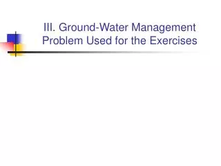
III. Ground-Water Management Problem Used for the Exercises. Ground-Water Flow System. The flow system is comprised of two confined aquifers separated by a confining unit.

E N D
Ground-Water Flow System • The flow system is comprised of two confined aquifers separated by a confining unit. • Inflow occurs primarily as areal recharge; there is also a very small amount of inflow across the boundary with the hillside. • At steady-state, outflow occurs only as discharge to the river.
Management Issues • Ground-water management issues related to this flow system: • Pumping wells for water supply are being completed in aquifers 1 and 2. The effect of pumping on the river is of concern, because there is a minimum required discharge from the ground-water system to the river. • A landfill is proposed in one corner of the study area. The landfill developers claim • (a) the landfill is outside the capture zone of the wells and • (b) any leaking effluent will reach the river sufficiently diluted. • We are developing a flow model to help evaluate these claims.
Predicted transport from landfill ? ? Will effluent go to well or river?
Ground-Water Flow Model • First, steady-state model without pumping will be developed and calibrated using available measurements of hydraulic-heads and discharge to the river, and will be used for preliminary evaluation of the issues. • Then, pumping wells will be installed, a long-term aquifer test will be conducted using the wells, and a transient model of the system will be recalibrated using the steady-state measurements as well as the additional drawdown and river discharge data collected during the test. • See flow model setup in Figure 2-1b (page 32) of Hill and Tiedeman. • See model parameter definition and starting values in Table 3-1 (page 38). • See true simulated conditions in Figures 2-1c and 2-1d (page 22-23).
MODFLOW Packages Used • Basic (BAS) and the Discretization input file • Define model grid, including rows, columns, and layers • Define types of model layer (confined; convertible) • Layer Property Flow (LPF) • Define hydraulic properties – K, Ss, Sy, Anisotropy • Recharge (RCH) • Define distribution of areal recharge • River (RIV) • General-Head Boundary (GHB) • Well (WEL) • Define pumpage • Used here for prediction runs only
Spatial Discretization -- Ground-Water Flow Model Grid Figure 2-1b of Hill and Tiedeman (page 22)
Layer-Property Flow Package Define hydraulic properties – K, Ss, Sy, Anisotropy Figure 2-1a of Hill and Tiedeman (page 34) Model layer 1 is homogeneous Model layer 2 has K that increases linearly from beneath the river to the hillside
Recharge Package • Can apply recharge to model layer 1 or top active cell at each row, column location • Input a flow rate (L/T). The program multiplies by area to get volume per time. • Layer data. • Parameters are used to define the recharge rate. • For this problem, use 2 zones; no multiplication arrays.
GHB The River (RIV) and General-Head Boundary (GHB)Packages are used • Both define head-dependent boundaries: q=C(H-h) RIV DRN
Well Package • List data – layer, row, column, pumpage rate • Input volume of discharge per time. Outflow is NEGATIVE. • For this problem, no pumpage parameters need to be defined, but you can use the parameter capability to define them if you like. [Why might you want to do that?]
Parameters and Starting Values Table 3-1 of Hill and Tiedeman (page 38)
True Simulated Conditions Figure 2-1 c and 2d of Hill and Tiedeman (page 22-23)
10 head observations, 5 in each model layer. Observed values shown in Table 3-2 (page 38) of Hill and Tiedeman. 1 steady-state flow observation: ground-water discharge to the river of –4.4 m3/sec. Observations
Well identifier Observation name Layer Row Col Observed head (m) Variance of well elevation measurement error (m2) Variance of water-level measurement error (m2) Variance of the observation (m2) 1 1.ss 1 3 1 101.804 1.00 0.0025 1.0025 2 2.ss 1 4 4 128.117 1.00 0.0025 1.0025 3 3.ss 1 10 9 156.678 1.00 0.0025 1.0025 4 4.ss 1 13 4 124.893 1.00 0.0025 1.0025 5 5.ss 1 14 6 140.961 1.00 0.0025 1.0025 6 6.ss 2 4 4 126.537 1.00 0.0025 1.0025 7 7.ss 2 10 1 101.112 1.00 0.0025 1.0025 8 8.ss 2 10 9 158.135 1.00 0.0025 1.0025 9 9.ss 2 10 18 176.374 1.00 0.0025 1.0025 10 10.ss 2 18 6 142.020 1.00 0.0025 1.0025 Head Observations Table 3-2 of Hill and Tiedeman (page 38)
Weighting is accomplished using UCODE_2005 • Here we break for a lecture introducing UCODE_2005
Weighted residuals are squared and summed in the objective function: Weights on Observations Heads Flows Prior • Need to weight the observations for two primary reasons: • So that residuals for observations with different units (e.g. heads and flows) can be summed in the objective function. • To account for different observations having different degrees of measurement error. Weighting is used to reduce the influence of observations that are less accurate, and to increase the influence of observations that are more accurate.
Defining the weights as being proportional to the inverse of the variance of measurement error meets both these needs: Weights on Observations • The variance of measurement error is an estimate of the uncertainty of the observation. How do we quantify this? • Need to quantify the uncertainty using: • A range that is symmetric about the measurement used for the observation. • A probability with which the true value is expected to occur within the range.
A head observation is thought to be “good to within 3 meters”. Quantify this as “there is a 95-percent chance the true value falls within 3 meters of the measurement.” Use a normal probability table to determine that a 95-percent confidence interval is a value plus and minus 1.96 times the standard deviation, . Thus, 1.96 x = 3 m, so = 1.53 m, and the variance 2 = 2.34 m2. Weights on Observations: Example 1
A measurement of stream loss to a ground-water system is derived by subtracting two streamflow measurements, an upstream value of 3.0 m3/s and a downstream value of 2.5 m3/s . Quantify uncertainty: The first measurement is considered to be slightly worse than the second. For the upstream measurement, the hydrologist believes that there is a 90% chance that the true value falls within ± 5% of the measured value; for the downstream measurement, there is a 95% chance that the true value falls within ± 5% of the measured value. Using values from a normal probability table, a 90% confidence interval is a value ±1.65 times the standard deviation, . Upstream measurement: 1.65 x = 0.05 x 3.0 m3/, so = 0.091 m3/s. Downstream measurement: 1.96 x = 0.05 x 2.5 m3/, so = 0.064 m3/s. The loss of streamflow in the reach between these two measurements is 0.5 m3/s. How accurately is this loss known? Add variances!! The variance of the loss is 0.0912 + 0.0642 = 0.0124 (m3/)2. Weights on Observations: Example 2
Head Observations: Elevation of each observation well has a variance of measurement error of 1.00 m2. Each water-level measurement has a variance of measurement error of 0.0025 m2. Thus, total variance measurement error = 1.0025 m2 Flow Observation: Coefficient of variation of 10%; thus = 0.1 x 4.4 m3/s = 0.44 m3/s DO EXERCISE 3.2d: Calculate weights on hydraulic-head and flow observations. Weights for the Steady-State Problem
From UCODE-2005 output file. DO EXERCISE 3.3: Evaluate model fit using the starting parameter values. Model Fit Using Starting Parameter Values DATA AT HEAD AND FLOW LOCATIONS OBSERVATION MEASURED SIMULATED WEIGHTED NAME VALUE VALUE RESIDUAL WEIGHT**.5 RESIDUAL hd01.ss 101.804 100.225 1.579 0.999 1.577 hd02.ss 128.117 139.331 -11.21 0.999 -11.20 hd03.ss 156.678 174.363 -17.68 0.999 -17.66 hd04.ss 124.893 139.331 -14.44 0.999 -14.42 hd05.ss 140.961 157.132 -16.17 0.999 -16.15 hd06.ss 126.537 139.632 -13.10 0.999 -13.08 hd07.ss 101.112 102.868 -1.756 0.999 -1.754 hd08.ss 158.135 173.956 -15.82 0.999 -15.80 hd09.ss 176.374 190.300 -13.93 0.999 -13.91 hd10.ss 142.020 157.041 -15.02 0.999 -15.00 flow01.ss -4.40000 -4.86060 0.4606 2.27 1.047 STATISTICS FOR THESE RESIDUALS: MAXIMUM WEIGHTED RESIDUAL: 0.158E+01 Observation: hd01.ss MINIMUM WEIGHTED RESIDUAL: -0.177E+02 Observation: hd03.ss AVERAGE WEIGHTED RESIDUAL: -0.106E+02 # RESIDUALS >= 0. : 2 # RESIDUALS < 0. : 9 NUMBER OF RUNS: 3 IN 11 OBSERVATIONS SUM OF SQUARED WEIGHTED RESIDUALS : 1752.4 SUM OF SQUARED WEIGHTED RESIDUALS WITH PRIOR: 1752.4 SUM OF SQUARED, WEIGHTED RESIDUALS: DEPENDENT VARIABLES: 1752.4 Least squares objective function
nh 2 å = w - S ( b ) ( h h ' ( b )) i i i = i 1 Example Least-Squares Objective Function HEADS FLOWS PRIOR
Basic Steps for Model Calibration Italicized steps are affected by using regression