Download
1 / 16
160 likes | 404 Views
Methods. Collect AWS observations from Antarctic-IDDDo subjective quality control remove obvious outliersCollect model time series from MM5 and WRF forecastsNear-surface dataModel integration time stepGrid point nearest AWS locationTemporally interpolate model output and observations to 10-m

E N D
1. Early comparison of MM5 and WRF time series to AWS observations
Kevin W. Manning
Mesoscale and Microscale Meteorology
Earth and Sun Systems Laboratory
National Center for Atmospheric Research
2. Methods Collect AWS observations from Antarctic-IDD
Do subjective quality control � remove obvious outliers
Collect model time series from MM5 and WRF forecasts
Near-surface data
Model integration time step
Grid point nearest AWS location
Temporally interpolate model output and observations to 10-minute intervals.
Plot the temperature and wind speed time series.
Two models
Two forecast cycles per day
5-day forecasts
20 different forecasts for any given observation time
Produce some simple statistics
Bias and RMSE as a function of forecast time
3. Caveats This study represents only the latest several weeks of data
Results and interpretation may turn out to be different for other seasons
MM5 and WRF are on similar grids, with similar terrain fields, but the configuration is not exactly the same
Differences in model output level:
MM5 output at lowest model level (~14 m AGL)
WRF output (diagnosed in PBL scheme) at 2 m (T) and 10 m (wind)
Think boundary-layer structure
Surface data offer a very limited look at model behavior
Think boundary-layer structure again
As always, the 0-36 hour of the 20-km grid, where nests are active, isn't straightforward to interpret, because of feedback from nests
Fix from a few days ago casts doubt on the WRF results
Heat flux between atmosphere and sub-surface levels was essentially shut down
4. Conclusions MM5 and WRF are comparable
Similar behavior and similar failings
Temperature:
Warm bias overall
WRF generally warmer than MM5
Can be a wide range of temperature values forecast for a given observation time
WRF seems to have more spread
Wind speed:
Wind events seem to be handled pretty well in both models
WRF generally has lower speed bias
We inherit some problems from the GFS initialization
Perhaps this contributes to our overall warm bias?
If we can address the warm bias, we would have a significant improvement in surface temperature forecasts
Possibilities:
Initialization
Ice temperatures, and initialization thereof
Ice, surface-layer physics, radiation, heat fluxes
Boundary layer structure, development of stable layer
5. Let�s get to the pictures
16. Discussion Useful statistics for forecasters?
Statistical correction to model time-series output?
Initialization
GFS � Too warm over plateau; too warm over Ross Ice Shelf
Ice temperature?
Warm bias on the plateau
Strategies to investigate and address?
Why such variability among forecasts?
Default Noah LSM setup probably not optimal for Antarctica
�Soil� characteristics?
Additional stations available in real time?