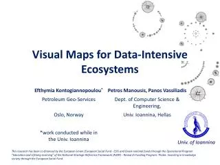
Visual Maps for Data-Intensive Ecosystems
Visual Maps for Data-Intensive Ecosystems. Univ. of Ioannina.

Visual Maps for Data-Intensive Ecosystems
E N D
Presentation Transcript
Visual Maps for Data-Intensive Ecosystems Univ. of Ioannina This research has been co-financed by the European Union (European Social Fund - ESF) and Greek national funds through the Operational Program ”Education and Lifelong Learning” of the National Strategic Reference Framework (NSRF) - Research Funding Program: Thales. Investing in knowledge society through the European Social Fund.
How do we make a map for a data-intensive software ecosystem? * *Information system with applications built around a central db and lots of queries blended in their code, thus having strong code-db dependencies
Why do we need these maps? • Documentation, • Program comprehension • impact analysis “Programmers spend between 60-90% of their time reading and navigating code and other data sources ... Programmers form working sets of one or more fragments corresponding to places of interest … Perhaps as a result, programmers may spend on average 35% of their time in IDEs actively navigating among working set fragments …, since they can only easily see one or two fragments at a time.” Bragdon et al. Code bubbles: rethinking the user interface paradigm of integrated development environments. ICSE (1) 2010: 455-464.
Circular placement for Drupal Hecataeustool: http://www.cs.uoi.gr/~pvassil/projects/hecataeus/
What happens if I modify table search_index? Who are the neighbors? Can play with the file structure too Hecataeustool: http://www.cs.uoi.gr/~pvassil/projects/hecataeus/
What happens if I modify table search_index? Who are the neighbors? Tooltips with info on the script & query + reporting at the “information area” Hecataeustool: http://www.cs.uoi.gr/~pvassil/projects/hecataeus/
So, … how do we make a map for a data-intensive software ecosystem?
A charting method for data-intensive ecosystems, with a clear target to reduce visual clutter. • We exploit a rigorous, graph-based model on code-db dependencies • modules (tables and queries embedded in the applications) as nodes and data provision relationships as edges • We cluster entities of the ecosystem in groups on the basis of their strong interrelationship • We chart the ecosystem via a set of radial methodsand provide solutions for • … cluster placement … • … node placement within clusters … • … tuning of visual representation details (shapes, colors, …) … all with the goal of reducing visual clutter
One (or more) embedding circle for cluster placement • Clusters are internally arranged over concentric circles, too • Node colors: acc. to script for queries; fixed for tables & views, • Node shape: relation / view / query • Node size: acc. to degree Graphical Notation The internal structure of a cluster Clusters • 4 bands of circles, within a cluster: • 1 circle for relations • As many as needed for views • 2 circles for queries … bioSQL Embedding circle
“Transparent” edges for less visual clutter • Edges are the main source of visual clutter! • So, we reduced the intensity of the edges’ presence of the visual map: • we picked a light gray color for the edges and • we made them very thin, in terms of weight (almost invisible). • To retain their info: every time a particular node is selected by the user its neighboring nodes are highlighted with a blue transparent color so, instead of emphasizing edges, we emphasize neighbors.
… and (finally) here is the method to construct the map: • Cluster similar nodes in groups (clusters) • A cluster is a set of relations, views and queries • Similarity is determined by the edges • Estimate the space required for each cluster • … to avoid cluster overlaps later • 3 alternative methods to place clusters on a 2D canvas • Single circle • Concentric Circles • Concentric Arcs • Place the nodes of each cluster in concentric circles, internally in the cluster
Roadmap 1. Cluster similar nodes in groups (clusters) 2. Estimate the space required for each cluster 3. Three alternative methods to place clusters on a 2D canvas • Single circle • Concentric Circles • Concentric Arcs 4. Place the nodes of each cluster in concentric circles, internally in the cluster 5. Summing up
Roadmap 1. Cluster similar nodes in groups (clusters) 2. Estimate the space required for each cluster 3. Three alternative methods to place clusters on a 2D canvas • Single circle • Concentric Circles • Concentric Arcs 4. Place the nodes of each cluster in concentric circles, internally in the cluster 5. Summing up
Step 1: Clustering • We use agglomerative hierarchical clustering to group objects with similar semantics in advance of graph drawing. • Why? To reduce the amount of visible elements,visualization methods place them in groups, thus • reducing visual clutter • improving user understanding of the graph • Principle of proximity: similar nodes are placed next to each other
Roadmap 1. Cluster similar nodes in groups (clusters) 2. Estimate the space required for each cluster 3. Three alternative methods to place clusters on a 2D canvas • Single circle • Concentric Circles • Concentric Arcs 4. Place the nodes of each cluster in concentric circles, internally in the cluster 5. Summing up
Step 2: Estimate the area of each cluster • Once the clusters have been computed, before placing them on the 2D canvas, the next step is to estimate the space required for each cluster • This step is crucial and necessary for the subsequent step of cluster placement, in order to be able to • calculate the radius and area each cluster, and thus, • arrange the clusters without overlaps
Step 2: Estimate the area of each cluster Εach cluster includes 3 bands of concentric circles: relations (1 circle), views, queries (2 circles) A cluster’s internal layout from the Biosql ecosystem
Step 2: Estimate the area of each cluster • We determine the clusters’ circles and their nodes: • We topologically sort cluster nodes in strata – each stratum becomes a circle • Then, we compute the radius for each circle: Ri = 3 * log(nodes) + nodes The outer circle gives us the radius of this cluster A cluster’s internal layout from the Biosql ecosystem
Roadmap 1. Cluster similar nodes in groups (clusters) 2. Estimate the space required for each cluster 3. Three alternative methods to place clusters on a 2D canvas • Single circle • Concentric Circles • Concentric Arcs 4. Place the nodes of each cluster in concentric circles, internally in the cluster 5. Summing up
Step 3: Laying out the Clusters 3 alternative methods for placing the clusters on a 2D area • Circular placement • all clusters on a single embedding circle • Concentric circles • trying to reduce the intermediate empty space • Concentric arcs • a combination of the previous two methods
Drupal Circular Layout bioSQL ZenCart OpenCart
Circular cluster layout • We use a single embedding circle to place the clusters. • One sector of the circle per cluster • with its angle varying on the cluster’s size (#nodes) • remember: each cluster is also a circle, approximated by its outermost constituent circle of nodes • Steps: • Compute R, the radius of the embedding circle • Compute φi, the angle of each cluster’s sector • Add some extra whitespace • Compute the coordinates of all clusters
compute R; compute φi; whitespace; coordinates. Circular Layout: Embedding Circle determination • Given: the radius ri of each cluster iCompute: R, the radius of the embedding circle. • Method: • approximate the circles periphery (2πR) by the sum of edges of the embedded polygon • divide this sum by 2π to calculate the radius R of the embedding circle
compute R; compute φi; whitespace; coordinates. Circular layout: calculation of the angle for each of the segments • Goal: assign each cluster to a segment of the circle depending on the cluster’s radius (size). • Each these segments is defined by an angle φover the embedding circle. • Not as obvious as it seems – we have to consider two cases: • The radius ρof the cluster we want to place is smaller or equal to the radius of the embedding circle R • The radius ρof the cluster we want to place is greater than the radius of the embedding circle R
compute R; compute φi; whitespace; coordinates. Circular layout: calculation of the angle for each of the segments • Typical case, where ≤ R • Consider the left triangle ABO • Then:
compute R; compute φi; whitespace; coordinates. Circular layout: calculation of the angle for each of the segments • A large cluster occurs > R • Assume the isosceles ABO, both AO,BO = R • Then: • due to Note: cannot avoid to discriminate the two cases
compute R; compute φi; whitespace; coordinates. Circular layout: avoid cluster overlap! original layout • We introduce a white space factor w that enlarges the radius R of the circle • Each cluster is approx. by a circle, with • radius r (known from step #1) • center [cx, cy] determined by φ, R, and w. extra whitespace
Drupal Concentric circles bioSQL ZenCart OpenCart
Concentric Circles Layout • Each circle is split in fragments of powers of 2 • as the order of the introduced circle increases, the number of fragments increases too (S = 2k), • with the exception of the outermost circle hosting the remaining clusters • This way, we can place • the small clusters on the inner circles, and • bigger clusters (occupying more space) on outer circles
Concentric Circles Layout Method: • Sort clusters by ascending size in a listLC • While there are clusters not placed in circles • Add a new circle and divide it in as many segments as S = 2k with k being the order of the circle (i.e., the first circle has 21 segments, the second 22 and so on) • Assign the next S fragments from the list LC to the current circle and compute its radius according to this assignment • Add the circle to a list L of circles • Draw the circles from the most inward (i.e., from the circle with the least segments) to the outermost by following the list L. Main challenge
Concentric Circles: radius calculation • Instead of having to deal with just one circle, we need to compute the radius for each of the concentric circles, in a way that clusters do not overlap • Overlap can be the result of two problems: • clusters of subsequent circles have radii big enough, so that they meet, or, • clusters on the same circle are big enough to intersect. R(Ki) = R(Ki-1) + Rmax(CKi-1)+Rmax(CKi)
Concentric Circles: radius calculation for each circle • Finally, to calculate the radius of a circle: • we take the maximum of the two values of the two aforementioned solutions and • we use an additional whitespace factor w to enlarge it slightly (typically, we use a fixed value of 1.2 for w). • Clustersof the same circle have equal segments with an angle: where n:the number of clusters on circle Ki
Concentric arcs Drupal bioSQL ZenCart OpenCart
Concentric Arcs Layout • To attain better space utilization • small clusters placed in the upper left corner • less whitespace to guard against cluster intersection • Just like concentric circles: • we deploy the clusters on concentric arcs Ai of size π/2 • we place 2i clusters on the ith arc • to avoid cluster overlaps, we use exactly the same radius optimization technique we used before. • Unlike the concentric circles, • the partition assigned to each cluster is proportionate to its size (as in the case of the single circle), again taking care to avoid overlaps
Roadmap 1. Cluster similar nodes in groups (clusters) 2. Estimate the space required for each cluster 3. Three alternative methods to place clusters on a 2D canvas • Single circle • Concentric Circles • Concentric Arcs 4. Place the nodes of each cluster in concentric circles, internally in the cluster 5. Summing up
Step 4: arrangement of nodes within the circular clusters Remember: 4 bands of circles to place nodes
Step 4: arrangement of nodes within the circular clusters • We want to follow a barycenter based method, which can work successfully for layered bipartite graphs • The standard barycenter method works with linear layers with the principle that once you have laid out layer i, you can lay out layer i+1 wrt the previous one • … practically placing nodes in the barycenter of their neighbors in the previous layer i • Here, we have two challenges: • adapt this to our radial, concentric circles • decide the initial order of the process (here: relations in the inner circle)
order R; place R & QR; place V & Q-QR. Step 4: arrangement of nodes within the circular clusters • Order the relations • Count the frequency of each combination of tables as hit by the queries • Place tables in popular combinations sequentially • Decide the position of relationsand relation-dedicated queries • Locate relation dedicated queries, decide the arc they need and position them sequentially • Place relation in the middle of this arc • Decide the position of the rest of the queries and the views • Stratify views and queries – each stratum has a dedicated circle • Place views and queries via a barycenter method on their angle • Adjust overlapping nodes (e.g., queries hitting exactly the same tables)
Roadmap 1. Cluster similar nodes in groups (clusters) 2. Estimate the space required for each cluster 3. Three alternative methods to place clusters on a 2D canvas • Single circle • Concentric Circles • Concentric Arcs 4. Place the nodes of each cluster in concentric circles, internally in the cluster 5. Summing up
Not covered in this talk / paper… • … failures & other tries …. • Algorithmic details and geometrical issues • … esp., concerning the intra-cluster placement • Relationship to aesthetic principles • Experiments To probe further (code, data, details, presentations, …) http://www.cs.uoi.gr/~pmanousi/publications/2014_ER/
We can tame code-db interdependence via rigorous modeling and visual methods • Visual methods to chart ecosystems explored on the grounds of: • … radial deployment • … grouping, coloring, placement • … visual clutter reduction • all aiming to better highlightcode-db relationships To probe further (code, data, details, presentations, …) http://www.cs.uoi.gr/~pmanousi/publications/2014_ER/
Why bother? • The problem is … • Important, as its implications relate to productivity and development effort • Hard to solve, not solved by SotA, as standard graph drawing methods do not seem to work well • Interesting, as it requires a large amount of technical solutions to visualization problems • … and, of course, we have not only solved it, but also, we have incorporated the solution to an actual system…
In a nutshell Fundamental modeling pillar: Architecture Graph G(V,E) of the data-intensive ecosystem. The Architecture Graphis a skeleton, in the form of graph, that traces the dependencies of the applicationcode from the underlying database. • modules (relations, viewsand queries) as nodes and • edges denoting data provision relationships betweenthem. Visualization choices: • Circular layout. Circular layouts give: • better highlight of node similarity, • less line intersections, i.e., less clutter • Clustered graph drawing. We place clusters of objects in the periphery of an embedding circle or in the periphery of several concentric circles or arcs. Each cluster will again be displayed in terms of a set of concentric circles, thus producing a simple, familiar and repetitive pattern.
One (or more) embedding circle for cluster placement • Clusters are internally arranged over concentric circles, too • Node colors: to which script queries belong • Node shape: relation / view / query Graphical Notation The internal structure of a cluster Clusters • 4 bands of circles, within a cluster: • 1 circle for relations • As many as needed for views • 2 circles for queries bioSQL Embedding circle
Aesthetics and design choices • Node shape: different shapes to visually distinguish the different type of nodes. Relation nodes have circular shape, view nodes have triangular shape and query nodes are depicted as hexagons. • Node size: scaled according to their node degree • the most used modules are more conspicuous. • Node color: we distinguish node types with different colors. • Relations are grey and views are dark green. (db’s are dark) • Querynodeshavedifferentcolors, depending on the folder their embedding script in the applications belongs. • Thus, the difference in color provides another way of grouping queries.
Visual clutter introduced by edges • Edges are the main source of visual clutter! • So, we reduced the intensity of the edges’ presence of the visual map: • we picked a light gray color for the edges and • we made them very thin, in terms of weight (almost invisible). • To retain their info: every time a particular node is selected by the user its neighboring nodes are highlighted with a blue transparent color so, instead of emphasizing edges, we emphasize neighbors.
Steps of the method Our method for visualizing the ecosystem is based on the principle of clustered graph drawingand uses the following steps: • Cluster the queries, views and relations of the ecosystem, into clusters of related modules. Formally, this means that we partition the set of graph nodes V into a set of disjoint subsets, i.e., its clusters, C1, C2, . . . , Cn. • Estimate the necessary area for each cluster. • Position the clusters on a two-dimensional canvas in a way that minimizes visual clutter and highlights relationships and differences. • For each cluster, decide the positions of its nodes and visualize it.