Petascale Data Intensive Computing for eScience
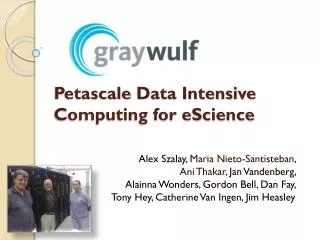
Petascale Data Intensive Computing for eScience. Alex Szalay, Maria Nieto-Santisteban, Ani Thakar, Jan Vandenberg, Alainna Wonders, Gordon Bell, Dan Fay, Tony Hey, Catherine Van Ingen, Jim Heasley. Gray’s Laws of Data Engineering. Jim Gray:

Petascale Data Intensive Computing for eScience
E N D
Presentation Transcript
Petascale Data Intensive Computing for eScience Alex Szalay, Maria Nieto-Santisteban, Ani Thakar, Jan Vandenberg, Alainna Wonders, Gordon Bell, Dan Fay, Tony Hey, Catherine Van Ingen, Jim Heasley
Gray’s Laws of Data Engineering Jim Gray: • Scientific computing is increasingly revolving around data • Need scale-out solution for analysis • Take the analysis to the data! • Start with “20 queries” • Go from “working to working” DISSC: Data Intensive Scalable Scientific Computing
Amdahl’s Laws Gene Amdahl (1965): Laws for a balanced system • Parallelism: max speedup is S/(S+P) • One bit of IO/sec per instruction/sec (BW) • One byte of memory per one instr/sec (MEM) • One IO per 50,000 instructions (IO) Modern multi-core systems move farther away from Amdahl’s Laws (Bell, Gray and Szalay 2006) For a Blue Gene the BW=0.001, MEM=0.12. For the JHU GrayWulf cluster BW=0.5, MEM=1.04
Commonalities of DISSC • Huge amounts of data, aggregates needed • Also we must keep raw data • Need for parallelism • Requests benefit from indexing • Very few predefined query patterns • Everything goes…. search for the unknown!! • Rapidly extract small subsets of large data sets • Geospatial everywhere • Limited by sequential IO • Fits DB quite well, but no need for transactions • Simulations generate even more data
Total GrayWulf Hardware • 46 servers with 416 cores • 1PB+ disk space • 1.1TB total memory • Cost <$700K
Data Layout • 7.6TB database partitioned 4-ways • 4 data files (D1..D4), 4 log files (L1..L4) • Replicated twice to each server (2x12) • IB copy at 400MB/s over 4 threads • Files interleaved across controllers • Only one data file per volume • All servers linked to head node • Distributed Partitioned Views
Software Used • Windows Server 2008 Enterprise Edition • SQL Server 2008 Enterprise RTM • SQLIO test suite • PerfMon + SQL Performance Counters • Built in Monitoring Data Warehouse • SQL batch scripts for testing • DPV for looking at results
Performance Tests • Low level SQLIO • Measure the “speed of light” • Aggregate and per volume tests (R, some W) • Simple queries • How does SQL Server perform on large scans • Porting a real-life astronomy problem • Finding time series of quasars • Complex workflow with billions of objects • Well suited for parallelism
IO Per Disk (Node/Volume) 2 ctrl volume Test file on inner tracks,plus 4K block format
Astronomy Application Data • SDSS Stripe82 (time-domain) x 24 • 300 square degrees, multiple scans (~100) • (7.6TB data volume) x 24 = 182.4TB • (851M object detections)x24 = 20.4B objects • 70 tables with additional info • Very little existing indexing • Precursor to similar, but much bigger data from Pan-STARRS (2009) & LSST(2014)
Simple SQL Query Harmonic Arithmetic 12,109 MB/s 12,081
Finding QSO Time-Series • Goal: Find QSO candidates in the SDSS Stripe82 data and study their temporal behavior • Unprecedented sample size (1.14M time series)! • Find matching detections (100+) from positions • Build table of detections collected /sorted by the common coadd object for fast analyses • Extract/add timing information from Field table • Original script written by Brian Yanny (FNAL) and Gordon Richards (Drexel) • Ran in 13 days in the SDSS database at FNAL
CrossMatch Workflow PhotoObjAll Field coadd 10 min filter filter zone1 zone2 join xmatch 2 min 1 min neighbors Match
Crossmatch Results • Partition the queries spatially • Each server gets part of sky • Runs in ~13 minutes! • Nice scaling behavior • Resulting data indexed • Very fast posterior analysis • Aggregates in seconds over0.5B detections Time [s] Objects [M]
Conclusions • Demonstrated large scale computations involving ~200TB of DB data • DB speeds close to “speed of light” (72%) • Scale-out over SQL Server cluster • Aggregate I/O over 12 nodes • 17GB/s for raw IO, 12.5GB/s with SQL • Very cost efficient: $10K/(GB/s) • Excellent Amdahl number >0.5
Test Hardware Layout • Dell 2950 servers • 8 cores, 16GB memory • 2xPERC/6 disk controller • 2x(MD1000 + 15x750GB SATA) • SilverStorm IB controller (20Gbits/s) • 12 units= (4 per rack)x3 • 1xDell R900 (head-node) • QLogicSilverStorm 9240 • (288 port IB switch)