Download
1 / 24
240 likes | 260 Views
This study explores forward detectors for luminosity measurement, discussing methods, requirements, and costs, aiming for high precision in cross-section comparisons and SUSY scenarios. It investigates optics solutions, roman pot detectors, luminosity monitors, and machine conditions for accurate measurements in various channels at the ATLAS experiment. The focus is on advancing optical theorems, dedicated luminosity monitors, and Coulomb scattering techniques to achieve the desired accuracy while addressing beam halo concerns and detector performance simulations.

E N D
ATLAS Forward Detectors for Luminosity Measurement and Monitoring Maarten Boonekamp, on behalf of the ATLAS coll. DIS 2004 Baseline Method and Requirements Optics Solution and Machine Conditions Roman Pot Detectors Luminosity Monitor LUCID Other Luminosity Methods Costs and Participants
Relative precision on the measurement of HBR for various channels, as function of mH, at Ldt = 300 fb–1. The dominant uncertainty is from Luminosity: 10% (open symbols), 5% (solid symbols). (ATL-TDR-15, May 1999) Luminosity Measurement • Goal: • Measure L with ≲2% accuracy • Luminosity needed for: • Precision comparison with theory: • bb, tt, W/Z, jet, …, H, SUSY, … • Cross sections gives additional info;will help disentangle SUSY scenarios • Precision comparison with other expt’s • Luminosity from: • LHC Machine parameters (~5-10%) • Optical theorem: forward elastic rate + total inelastic rate: needs ~full |η| coverage • Rates of well-calculable processes:e.g. QED, QCD, • need DEDICATED Luminosity monitor
Need to reach tmin0.01 GeV2 L from the Optical Theorem • Luminosity from the machine: accuracy goal 5%, probably limited by: • extrapolation of x , y (or , x , y) from measurements of beam profiles elsewhere to IP • beam-beam effects at IP, effect of crossing angle at IP, … • Van der Meer scans à la ISR? Cross checks with HI running? • Using the Optical Theorem and the total inelastic rate: (Method pursued by TOTEM/CMS) • ATLAS does NOT have sufficient forward coverage to measure Ninel well enough… = =
Luminosity from Coulomb Scattering • Elastic scattering at micro-radian angles: • Required reach in t:tmin-t(|fC|=| fN|) 8EM/tot 6×10⁻⁴ GeV2 θmin 3.5 μrad • Requires: • small intrinsic beam angular spread at IP small emittance • detectors close to the beam, at large distance from IP • parallel-to-point optics, insensitive to transverse vertex smearing and with large effective lever arm Leff =
Experimental Technique • independence of vertex position: • parallel-to-point focusing:ydet = M11,yy* +M12,y y*with:M11,y = (/*) [cosy *siny] ( ψ(s) ≡0∫sds/β(s) )M12,y = (*) siny(* = value at IP)optimum: M11= 0, M12 large: sit at y(s) = (n ½), n=0,1,2,… and make * 0, * largethen: ydet = M12 y* = (*) y* = Leff,yy* • limit on minimum |t|min: *min = dmin/Leff, tmin = (*min pb)2 , with dmin = nσy = nσ(N/γ)tminpb2nσ2(N/γ) /* Thus: maximize *; minimize nσ and N parallel-to-point focusing ydet y* y* s IP Leff
(RA LHC MAC 13/3/03) nσ-reach? Beam Halo: limit on nσ • Beam halo is a serious concern for Roman Pot operation • determines the distance of closest approach dminof (sensitive part of) detector: nσ = dmin/σbeam: 9 ≤ nσ≤ 15 • expected halo rate (43 bunches, Np=1010, εN = 1.0 μm, nσ=10): 6 kHz
Emittance • Emittance can be reduced to 1.0×10⁻⁶ m (std: 3.75×10⁻⁶ m) • Recent LHC information: emittance εN, number of protons/bunch Np , and collimator opening nσ,coll (in units of σ) are related via a resistive (collimator) wall instability limit criterion: • Thus: εN ≥ 1.5×10⁻⁶ m (for Np=1010, nσ,coll=6 ) • For nσ=10: if tmin= pb2nσ2ε/β*≤ 4×10⁻⁴then: β*≳ 2500 m • beam size at detector: d = √(βdεN/γ) , • Beam safety: kσd≳ 1.0-1.5 mm then: βd≳ 100 m
2625 m Optics (A. Faus-Golfe et al.) • Smooth path to injection optics exists • All Quads are within limits • Q4 is inverted w.r.t. standard optics! β [m] D [m] }Leff
Roman Pot Locations TOTEM Pot 240 m
Requirements for Roman Pot Detectors • “Dead space”d0 at detector’s edge near the beam the beam: d0≲ 200 m (full/flat efficiency away from edge) • Detector resolution: d = 30 m • Same d = 30 m relative position accuracy between opposite detectors (e.g. partially overlapping detectors, …) • Radiation hardness: 100 Gy/yr • Operate with the induced EM pulse from circulating bunches (shielding, …) • Rate capability: O(Mhz) (40 MHz); time resolution t = O(1 ns) • Readout and trigger compatible with DAQ • Other: • Simplicity, Cost • extent of R&D needed, time scale, manpower, … • issues of LHC safety and controls
Roman Pot Detectors • Square scintillator strips • Kuraray 0.5 mm× 0.5 mm • 10 layers per coordinate • 50 μm offset between layers • Readout: • MultiAnode PMT, or • Avalanche Photodiodes • Trigger: • scintillator panes (possibly subdivided?) • Trigger latency: MARGINAL! p from IP RP: 800 ns signal RP CTP: 1000 ns trigger formation: 100 ns TOTAL: 1900 ns > 1.8μs remains to be sorted out… halo inter calibration planes (well away from beam)
Detector Performance Simulations • first simulation results: • strip positioning σfiber ≈ 20 μm • light and photo-electron yield:Npe = <dE/dx> dfiber (dnγ/dE) εAεTεCgRεQεd≈ 5 p.e. marginal !
Track traversing the fiber planes. The detection efficiency/fiber is 95%. All 10 hit fibers and the 30 multiplexed fibers give a signal. The hits of the 10 planes are projected in a histogram. The real hits can clearly be distinguished from the randomly distributed multiplexed hits. Tracking Simulation (multiplexing) • normal incidence tracks; assume: • fiber readout multiplexing (4/1) • fiber position smearing: 20 μm • fiber efficiency 85-95% Spatial resolution of a fiber plane for a detection efficiency per fiber of 85%. On average 8.2 fibers are hit (plus 24.6 multiplexed fibers). The Gaussian fit indicates a resolution of 25.4 mm.
Proof of Principle (M. Haguenauer et al.) • Test beam hodoscope : • 1x1 mm2 • multiplexed MAPMT readout Fibres KURARAY amoy=0,5 mm ± 0,06 mm bmoy=0,05 mm ± 0,01 mm a b a b
Luminosity Performance Simulations • Baseline optics, with baseline detector resolutions • smearing of hits on the detector plane caused by • detector resolution (30 μm) – negligible contribution • beam angular spread (σθ* = 0.23 μrad) • transverse vertex smearing (σ* = 0.42 mm), • vertical coordinate: σ(y) = 0.23 μrad × 563 m = 127 μmvertical smearing reduces acceptance near the detector edge • horizontal coordinate: σ(x) = 0.23 μrad × 143 m 0.42 mm × 0.168 = 32 μm 71 μm = 87 μmNote: taking the combination of left and right arms, the vertex smearing drops out (there is no detector edge in x!)
Simulated Elastic Scattering • Inner ring: t = -0.0007 GeV2 • Outer ring: t = -0.0010 GeV2 • Reconstruct θ*:
Simulated dNel/dt and Naïve Fit • 10 M evts with±45° fiducial cut on φ* • NO systematics on beam optics! • Only 1 station/arm 5M events Generated ~90 hr at L=1027 cm-2s-1 Fit Results (χ2/NDF=1442/1467):σtot = 98.7±0.8 mb (100)ρ = 0.148±0.007 (0.15)B = 17.90±0.12 GeV-2(18)L = (1.11±1.6%) 1027cm-2s-1 (1.09×1027) Range for fitting: 0.00056 <|t|<0.030 GeV2↖ (pθmincos45º)2 ~4M events ‘Measured’ dN/d|t|
Luminosity Monitoring • LUCID: (Jim Pinfold et al.: Alberta, Lund, Montreal, Regina, Saclay) • Dedicated detector: • bundle of projective Cerenkov cones: 5 layers of 40 tubes each • low mass (6 kg), rad hard (C4F10 gas?), quartz fiber readout • 40 MHz capability: • linearity required over 2x10⁻⁴ – 20 interactions/crossing • Cross-Calibration at low L = 1027: • non-beam-beam backgrounds, e.g. beam-gas, can be important at low L!! • Counts primary particles (only Č-photon statistics) • Mostly insensitive to non-primary particles • total signal #charged prim’s interactions/crossing L • LUCID should operate at start-up (machine diagnostics) • can be calibrated absolutely later… • may be used in rapidity-gap vetoing (under study), etc… • proof of principle: CLC at CDF! (e.g. S. Klimenko et al., NIM A441 (2000) 266) • Preliminary approval by ATLAS last year
ATLAS – Luminosity Monitor (J. Pinfold et al.) Services In/Out To UXA PMTs LUCID ~17< |z| <~18.5 m 5.4< || <6.1 Inner radius of LUCID ~8 cm, outer radius ~16cm
LUCID - Simulation Geant4 Simulation:Variation of #photons vs. muon incidence angle (measured at the tube centre) ~2 cmØ,1.5m tubes Front (J. Pinfold et al.) Rear – Showing Winston Cones #photons/20 GeV μ at photo-detector: 70(1.5 m Č) x0.8(Cone acc.) x0.6(Fiber acc.) x0.4(att. 20 m fiber) = 15 prototypes Aug’03
Lucid Performance Simulations • PYTHIA-6(MSEL=2, MSUB995)=1, MSTP(82)=0)events generated with increasing numbers of pile-up events • Perfect linearity, with little sensitivity for secondaries • Proof of Principle: the CDF CLC device Number of Axi-Linear Tracks/Crossing/Arm single track/tube peak Number of Interactions/Crossing
Cross Calibration • CNI calibration: L = 1028 cm–2s–1 (~2×10⁻⁴ evts/crossing) • Standard runs: L = 1033-34 cm–2s–1 • LUCID resolves bunches: calibration must be transferred from 2×10⁻⁴ to about 20 evts/crossing • Thus: non-beam-beam background rejection must be excellent at low L; note: beam-gas Np; beam-beam Np2 • Remains to be studied in detail!
L from other Physics Signals Use well-calculable QED/QCD signals as Physics Monitors:L 2-4% • QED: pp (p+*)+(p+*)p+()+p (A.Shamov & V.Telnov, hep-ex/0207095) • Signal: (μμ)-pair with |η(μ)|<2.5, pT(μ)≳ 5-6 GeV, pT(μμ) ≃ 0 • small rate ~1pb (~0.01 Hz at L=1034) off-line: preliminary estimate δL ≃ 2% for 10 fb–1 • Clean: backgrounds from DY, b,c-decays: handled by appropriate offline cuts. • uncertainties: μ trigger acceptance & efficiency, … • Full simulation studies in progress (Alberta, SACLAY) • QCD: W/Zleptons(Dittmar, Pauss, Zurcher, PRD56 (1997) 7284) • High rate:Wlν : ~60 Hz at L=1034 (ε=20%) • Gives relevant parton luminosity directly… • Current “theory” systematics: σW/Z 4% (V. Khoze et al., hep-ph/0010163) • Detection systematics: • Trigger/Selection eff’s, Backgrounds (and L-dependence) seem manageable • Detailed study for ATLAS detector needed (Alberta, SACLAY) Both processes will be used – at very least as cross checks…
Summary • ATLAS aims to determine absolute L in special high-β* runs measuring Coulomb scattering • The CNI normalization is verychallenging but seems attainable in principle – critically dependent on control of the beam and backgrounds • Roman Pot detectors: no show stoppers • This normalizes a dedicated L-monitor: the Č-detector LUCID • LUCID prototyping is well underway: no show stoppers • Other processes will be employed as well: • W/Z production, • double-photon exchange di-muon production, • machine L measurements, aided by HI experience… • … • Experience with RPs will help us prepare expansion of the ATLAS program with Central and Forward Diffraction…