6 th Homework - Solution

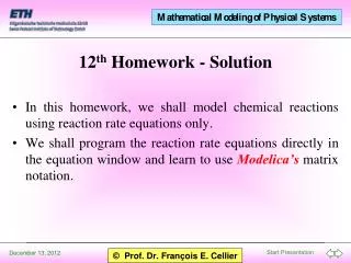
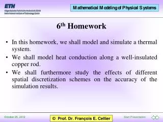
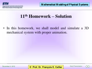
1. In this homework, we shall model and simulate a thermal system. We shall model heat conduction along a well-insulated copper rod. We shall furthermore study the effects of different spatial discretization schemes on the accuracy of the simulation results. 6th Homework - Solution

2. Heat conduction in copper rod Influence of asymmetric entropy feed Influence of discretization

3. A copper rod of length l = 1 m with a radius of r = 1 cm is initially in thermo-dynamical equilibrium at T = 298K. At Time = 0, the left end of the rod is brought in contact with a body that had been pre-heated to a temperature of TL = 390K. We wish to model the rod using 10 segments,eachwith a length of Dx = 10 cm. The boundary conditions are to be modeled such that the body to the left is replaced by a temperature source. It is assumed that no heat flows out at the right end of the rod, and that the rod is thermally so well insulated that no heat is lost anywhere along the rod. Heat Conduction in a Copper Rod I

4. The density of copper is r = 8960 kg·m-3. Its specific thermal conductivity is l = 401 J ·m-1 ·s-1 ·K-1. Its specific heat capacity is c = 386 J·kg-1·K-1. The heat conduction is modeled using the symmetric heat conduction element presented in class. This element is made available as part of the BondLib thermal sub-library. Simulate the system during 5 hours. Heat Conduction in a Copper Rod II

5. T ΔT Let us start by looking at some thermal models in the Dymola BondLib library that we haven‘t used before. These are stored in its thermal sub-library.

6. T

7. ΔT ΔT T1 T2 ΔT T2 T2 T1 T1 Compensation of the split feedback. Model class HE Model class HEr

8. The 0 on the right is contained in the model, the one one the left isn’t. In this way, elements can be cascaded. The capacity obtains here its initial condition. We can now start creating the individual chain links.

9. The initial condition is passed on as a parameter.

10. Heating element on the left Insulation on the right

11. Symmetric heat conduction Asymmetric heat conduction with preference to the right Asymmetric heat conduction with preference to the left

12. Here, the parameters  and  are computed. Modelica allows to compute parameter values.

13. Temperature values as functions of time and space 20 cm 40 cm 60 cm 80 cm 1 m

14. Replace the symmetric heat conduction element by two asymmetric elements; one, in which the generated entropy is fed only to the right, the other, in which it is fed exclusively to the left. The BondLib library offers such an element as well. Simulate the so modified model, and present, on a single plot, the results of the three simulation models. You may either calculate the three models sequentially while preserving the results from one to the next, or you may simulate the three models in parallel. Influence of Asymmetric Entropy Feed

15. Three independent models computed in parallel Asymmetric heat conduction with preference to the left Symmetric heat conduction Asymmetric heat conduction with preference to the right

16. We return to using the symmetric model. However this time, we wish to model the system using 20 segments, each with a length of Dx = 5 cm. Simulate the so modified model, and present the results obtained in this way graphically together with the original simulation results. Influence of Discretization

17. Discretized using 20 segments Discretized using 10 segments