Download
1 / 27
300 likes | 562 Views
METHOD OF STEEPEST DESCENT. Mean Square Error (Revisited). For a transversal filter (of length M), the output is written as and the error term wrt. a certain desired response is . Mean Square Error (Revisited). Following these terms, the MSE criterion is defined as

E N D
METHOD OF STEEPEST DESCENT ELE 774 - Adaptive Signal Processing
Mean Square Error (Revisited) • For a transversal filter (of length M), the output is written as and the error term wrt. a certain desired response is
Mean Square Error (Revisited) • Following these terms, the MSE criterion is defined as • Substituting e(n) and manupulating the expression, we get where Quadratic in w !
Mean Square Error (Revisited) • For notational simplicity, express MSE in terms of vector/matrices where
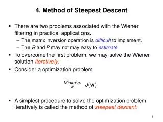
Mean Square Error (Revisited) • We found that the solution (optimum filter coef.s wo) is given by the Wiener-Hopf eqn.s • Inversion of R can be very costly. • J(w) is quadratic in w→ convex in w → for wo, • Surface has a single minimum and it is global, then • Can we reach to wo, i.e. with a less demanding algorithm?
Basic Idea of the Method of Steepest Descent • Can we find wo in an iterative manner?
Basic Idea of the Method of Steepest Descent • Starting from w(0), generate a sequence {w(n)} with the property • Many sequences can be found following different rules. • Method of steepest descent generates points using the gradient • Gradient of J at point w, i.e. gives the direction at which the function increases most. • Then gives the direction at which the function decreases most. • Release a tiny ball on the surface of J → it follows negative gradient of the surface.
Basic Idea of the Method of Steepest Descent • For notational simplicity, let , then going in the direction given by the negative gradient • How far should we go in –g → defined by the step size param. μ • Optimum step size can be obtained by line search - difficult • Generally a constant step size is taken for simplicity. • Then, at each step improvement in J is (from Taylor series expansion)
Application of SD to Wiener Filter • For w(n) • From the theory of Wiener Filter we know that • Then the update eqn. Becomes which defines a feedback connection.
Convergence Analysis • Feedback → may cause stability problems under certain conditions. • Depends on • The step size, μ • The autocorrelation matrix, R • Does SD converge? • Under which conditions? • What is the rate of convergence? • We may use the canonical representation. • Let the weight-error vector be then the update eqn. becomes
Convergence Analysis • Let be the eigendecomposition of R. • Then • Using QQH=I • Apply the change of coordinates • Then, the update eqn. becomes
Convergence Analysis • We know that Λ is diagonal, then the k-th natural mode is or, with the initial values vk(0), we have • Note the geometric series
Convergence Analysis • Obviously for stability or, simply • Geometric series results in an exponentially decaying curve with time constant τk, where letting or
Convergence Analysis • We have but We know that Q is composed of the eigenvectors of R, then or • Each filter coefficient decays exponentially. • The overall rate of convergence is limited by the slowest and fastest modes then
Convergence Analysis • For small step size • What is v(0)? The initial value v(0) is • For simplicity assume that w(0)=0, then
Convergence Analysis • Transient behaviour: • From the canonical form we know that • then • As long as the upper limit on the step size parameter μ is satisfied, regardless of the initial point
Convergence Analysis • The progress of J(n) for n=0,1,... is called the learning curve. • The learning curve of the steepest-descent algorithm consists of a sum of exponentials, each of which corresponds to a natural mode of the problem. • # natural modes = # filter taps
Example • A predictor with 2 taps (w1(n) and w2(n)) is used to find the params. of the AR process • Examine the transient behaviour for • Fixed step size, varying eigenvalue spread • Fixed eigenvalue spread, varying step size. • σv2 is adjusted so that σu2=1.
Example • The AR process: • Twoeigenmodes Conditionnumber (Eigenvalue Spread):
Example (Experiment 1) • Experiment 1: Keep the step size fixed at • Change the eigenvalue spread
Example (Experiment 2) • Keep the eigenvalue spread fixed at • Change the step size (μmax=1.1)
Example (Experiment 2) • Depending on the value of μ, the learning curve can be • Overdamped, moves smoothly to the min. ((very) small μ) • Underdamped, oscillates towards the min. (large μ< μmax) • Critically damped • Generally rate of convergence is slow for the first two.
Observations • SD is a ‘deterministic’ algorithm, i.e. we assume that • R and p are known exactly. • In practice they can only be estimated • Sample average? • Can have high computational complexity. • SD is a local search algorithm, but for Wiener filtering, • the cost surface is convex (quadratic) • convergence is guaranteed as long as μ< μmax is satisfied.
Observations • The origin of SD comes from the Taylor series expansion (as many other local search optimization algorithms) • Convergence can we very slow. • To speed up the process, second term can also be included as in the Newton’s Method • High computational complexity (inversion), numerical stability problems. Hessian