Introduction to PID Control: Understanding Controllers and Tuning Techniques
1.23k likes | 1.3k Views
Learn the fundamentals of PID control, including the UNICOS PID controller, manual tuning, autotuning, and control system design. Explore key concepts such as setpoint, control input, feedback, and error signal. Understand the challenges and solutions in proportional control and steady-state error. Enhance your skills with practical exercises and Q&A sessions.

Introduction to PID Control: Understanding Controllers and Tuning Techniques
E N D
Presentation Transcript
Introduction to PID Control Brad Schofield, BE ICS AP Brad Schofield
Course plan Document reference 09:00-10:00: What is PID control? 10:00-10:30: The UNICOS PID controller 10:30-10:45: Coffee 10:45-11:15: Manual tuning 11:15-12:00: Manual tuning exercise 12:00-14:00: Lunch 14:00-15:00: Autotuning 15:00-16:00: Autotuning exercise 16:00-16:15: Coffee 16:15-17:00: Questions & Wrap-up
What is PID Control? Document reference • Let’s take a step back… What is control? • Control is just making a dynamic process behave in the way we want • We need 3 things to do this: • A way to influence the process • A way to see how the process behaves • A way to define how we want it to behave
Defining behaviour Document reference • We usually specify a value we want some output of the system to have • Usually called the Setpoint (SP) • Can be the temperature of a room, the level in a tank, the flow rate in a pipe… • The value can be fixed, or may change with time…
Influencing the process Document reference We need some kind of control input which can create changes in the behavior of the process Can be a heater, a valve, a pump… Typically it is not the same physical quantity as what we are controlling
Observing behavior Document reference • If we knew exactly how the process worked, we would know what the output would be for a given control input… • Most of the time we don’t know exactly, so we need to measure what the process does • Usually called Measured Variable (MV) or Process Variable (PV)
Feedback Control Document reference Now we have a measurement (MV), some value that we want it to be (SP), and some way to make changes to the process (control input) We can ‘close the loop’
The Controller as a System SP Controller Control MV Document reference Now we can see that any controller can be thought of as a system that takes a setpoint and a measured value as inputs, and gives a control signal as an output
The Controller as a System SP Controller Control MV Document reference The controller needs to convert two signals of one physical quantity (such as temperature) into one signal of another (such as valve position)
The Controller as a System Document reference • We know that the process is a dynamic system: • Its outputs depend on current inputs as well as its past state • For the controller to deal with this, it makes sense that it should be a dynamic system too
The Error Signal Error + Σ Controller - SP Control MV Document reference Very often we can think of the controller acting on the difference between SP and MV:
The Closed Loop Process e u + Σ - Controller SP MV Document reference This is the ‘classic’ closed loop block diagram representation of a control system
A Dynamic Controller Document reference • We said that since the process is dynamic (dependent on inputs made at different times), it makes sense that the controller should be too • How do we usually think of time? • ‘Present’ • ‘Past’ • ‘Future’
Splitting the Controller Present Process u e + Σ Past - Future SP MV Document reference
The ‘Present’ Document reference This part of the controller is only concerned with what the error is now Let’s take a simple law: let the control signal be proportional to the error:
Proportional Control Document reference This is what is referred to as proportional control. The control action at any instant is the same as a constant times the error at the same instant The constant is the Proportional Gain, and is the first of our controller’s parameters
Proportional Control Proportional Process u e + Σ Past - Future SP MV Document reference
Is Proportional Control enough? Document reference Intuitively it seems like it should be fine on its own: when the error is big, the control input is big to correct it. As the error reduced so does the control input. But there are problems…
Problem 1 Think of a pendulum. If the setpoint is hanging straight down, then gravity acts as a proportional controller for the position… Pendulum will oscillate! Document reference
Problem 2 • What happens when the error is zero? • Control input is zero. • Causes problems if we need to have a nonzero control value while at our setpoint Document reference
Problem 2: steady state error This problem is normally called steady state error It’s a confusing name. The issue is just that the controller can’t produce any output when the error is zero. Easiest to see for tank level control: If there is a constant flow out of the tank, the controller must provide the same flow in, while the level is at the setpoint. Document reference
Problem 2: steady state error With P control, once the error has reached a value where is equal to the flow out, the level will stabilize. But it will be different to the setpoint Document reference
P control problem summary • Problem 1: oscillations • P control will give us oscillations in some processes, regardless of the value of the gain parameter. • Problem 2: steady state error • P control cannot give us a nonzero value of the control at zero error for some types of process Document reference
Solving P control’s problems Document reference How to get rid of steady state error? Let’s ignore the present for the moment and concentrate on what has happened in the past
Solving steady state error: ‘the Past’ Proportional Process u e + Σ Past - Future SP MV Document reference Let’s look at the error in the past
Solving steady state error We can examine how the controller error has evolved in the past If we sum up the past values of the error, we can get a value that increases when there is a constant error Document reference
Integral Action Document reference We can let the control be given by the sum of past values of the error, scaled by some gain. In continuous time the sum is an integral:
Integral Action Proportional Process u e + Σ Integral - Future SP MV Document reference
Integral gain, Integral time Document reference Here is where confusion can start… We have an integral gain which converts an integrated error to a control signal We would actually like to parameterize this as a time, as in how fast we can remove a steady state error
Integral gain, Integral time Document reference Let’s rewrite: As: is our Proportional Gain, and is our Integral Time
The Integral time Document reference Why do we use both and here? Let’s add the proportional and integral parts:
Proportional and Integral Controller Proportional Process u e + Σ Integral - Future SP MV Document reference
Proportional and Integral Controller = PI Controller Document reference We can rewrite the control law: is the gain parameter, is the time it takes to fix a steady state error
Solving P control’s problems revisited Document reference We solved the steady state error by adding integral action (summing the past) How can we solve the oscillation problem? Let’s look at the future!
Solving oscillations: ‘the Future’ Proportional Process u e + Σ Integral - Future SP MV Document reference Let’s look at the error in the future
Solving oscillations: ‘the Future’ How do we predict the future of the error? Look at its gradient! If the gradient (the time derivative) of the error is in a direction that makes the error smaller, we can reduce the control input Document reference
Damping It can be easier to think of this as damping, something that resists velocity Think of the wheel on your car… Document reference
Damping The spring is a proportional controller for the wheel position. The damper adds a derivative action by opposing the velocity of the wheel Document reference
Derivative action Document reference Let’s let the control be dependent on the derivative of the error: Here is the derivative gain. Let’s again split this into , where is the derivative time
Derivative action Proportional Process u e + Σ Integral - Derivative SP MV Document reference
PID Controller! Proportional Process u e + Σ Integral - Derivative SP MV Document reference
Derivative Time Document reference Why do we want as a parameter? We can think of it as how far ahead we want to predict! Easier to relate to process
Problems with Derivative action We know that a derivative amplifies quick changes. We can get problems if MV is noisy. Solution is to add low pass filter Document reference
Derivative with filter Document reference We already have: Equations will get messy if we add a filter in time domain! Let’s use Laplace! Then we can use algebra instead of calculus.
Derivative with filter Document reference Laplace transform frequency variable s is also an operator. Multiplication by s is derivation, and division is integration. So the derivative part is now
Derivative with filter Document reference We add a low pass filter: Now we have another parameter which is the filter bandwidth. So introducing derivative action requires two more parameters!
Full PID equation Document reference The complete PID controller now looks like:
Full PID equation Document reference This simplifies to:
ISA PID Form Document reference This is the ISA ‘standard form’ for a PID We have one gain, and three time constants