PID control. Practical issues
PID control. Practical issues. Smith Predictor (NOT PID…) PID Controller forms Ziegler-Nichols tuning Windup Digital implementation. TexPoint fonts used in EMF. Read the TexPoint manual before you delete this box.: A A A A A A A A A. Smith Predictor. PID controller. “Ideal” form:.

PID control. Practical issues
E N D
Presentation Transcript
PID control.Practical issues Smith Predictor (NOT PID…) PID Controller forms Ziegler-Nichols tuning Windup Digital implementation TexPoint fonts used in EMF. Read the TexPoint manual before you delete this box.: AAAAAAAAA
PID controller “Ideal” form: • e(t) = ys – ym(t) • P-part: MV (Δu) proportional to error • This is is main part of the controller! • I-part: To avoid offset, add contribution proportional to integrated error. • Integral keeps changing as long as e≠0 • -> Will eventually make e=0 (no steady-state offset!) • Possible D-part: Add contribution proportional to change in (derivative of) error • Can improve control for high-order (S-shaped) response, but sensitive to measurement noise
“Ideal” PID (parallel form) 1. To get realizable controller and less sensitivity to measurement noise: replace ¿D s by 2. To avoid “derivative kick” do not take derivative of setpoint 3. To avoid integral “windup” when input saturates (at max or min), use “anti” windup. Simplest: Stop integration while input saturates
Block diagram of practical “ideal” PID ys u For smoother control/ less sensitivity to noise + : Replace ¿D s by ¿D s /(α¿Ds +1) 2. To avoid “derivative kick” : Do not take derivative of setpoint ys y
Series (cascade) PID Typical: ®=0.1 u ys y For smoother control: Replace (¿Ds+1) by (¿D s +1)/(α¿Ds +1) 2. To avoid “derivative kick” do not take derivative of setpoint
Series to ideal form Derivation: See exercise Note: The reverse transformation (from ideal to series) is not always possible because the ideal controller may have complex zeros.
Optimal PID settings • Can find optimal settings using optimization • SIMC-rules are close to IAE-optimal for combined setpoints and disturbances* *Chriss Grimholt and Sigurd Skogestad. "Optimal PI-Control and Verificationofthe SIMC Tuning Rule".ProceedingsIFAC conferenceonAdvances in PID control(PID'12), Brescia, Italy, 28-30 March 2012.
Methods for online tuning of PID controllers • Trial and error • Ziegler Nichols • Oscillating P-control • Relay method to get oscillations • Closed-loop response with P-control • Shams method On-line tuning: Avoids an open-loop experiment, like a step input change. Advantage on-line: Process is always “under control” In practice: Both “open-loop” and “closed-loop” (online) methods are used
Tuning of your PID controllerI. “Trial & error” approach (online) • P-part: Increase controller gain (Kc) until the process starts oscillating or the input saturates • Decrease the gain (~ factor 2) • I-part: Reduce the integral time (I) until the process starts oscillating • Increase a bit (~ factor 2) • Possible D-part: Increase D and see if there is any improvement Very common approach, BUT: Time consuming and does not give good tunings: NOT recommended
II. Ziegler-Nichols closed-loop method (1942) • P-control only: Increase controller gain (Kc) until the process cycles with constant amplitude: • Write down the corresponding “ultimate” period (Pu) and controller gain (Ku). • Based on this “process information” obtain PID settings: ZN is often a bit aggressive. TL-modification is smoother (smaller Kc and larger ¿I). (ideal)
TIGHT CONTROL Example. Integrating process with delay=1. G(s) = e-s/s. Model: k’=1, =1, 1=1 SIMC-tunings with c with ==1: IMC has I=1 Ziegler-Nichols is usually a bit aggressive Setpoint change at t=0c Input disturbance at t=20
TIGHT CONTROL • Approximate as first-order model with k=1, 1 = 1+0.1=1.1, =0.1+0.04+0.008 = 0.148 • Get SIMC PI-tunings (c=): Kc = 1 ¢ 1.1/(2¢ 0.148) = 3.71, I=min(1.1,8¢ 0.148) = 1.1 2. Approximate as second-order model with k=1, 1 = 1, 2=0.2+0.02=0.22, =0.02+0.008 = 0.028 Get SIMC PID-tunings (c=): Kc = 1 ¢ 1/(2¢ 0.028) = 17.9, I=min(1,8¢ 0.028) = 0.224, D=0.22
Åstrøm relay method (1984): Alternative approach to obtain cycling (and Ku+Pu) • Avoids operating at limit to instability • Use ON/OFF controller (=relay) were input u(t) varies § d (around nominal) • Switch when output y(t) reaches §a0(deadband) (around setpoint) • Example: Thermostat in your home • From this obtain Pu and d: amplitude u(t) (set by user) a: amplitude y(t) (from experiment)
Alternative to Ziegler-Nichols closed-loop experiment that avoids cycling. III. Shams’ method: Closed-loop setpoint response with P-controller with about 20-40% overshoot Kc0=1.5 Δys=1 Δy∞ OBTAIN DATA IN RED (first overshoot and undershoot), and then: dyinf= 0.45*(dyp + dyu) Mo =(dyp -dyinf)/dyinf % Mo=overshoot (about 0.3) b=dyinf/dys A = 1.152*Mo^2 - 1.607*Mo + 1.0 r = 2*A*abs(b/(1-b)) 2. OBTAIN FIRST-ORDER MODEL: k = (1/Kc0) * abs(b/(1-b)) theta = tp*[0.309 + 0.209*exp(-0.61*r)] tau = theta*r 3. CAN THEN USE SIMC PI-rule Δyp=0.79 Δyu=0.54 tp=4.4 Example 2: Get k=0.99, theta =1.68, tau=3.03 Ref: Shamssuzzoha and Skogestad (JPC, 2010) + modification by C. Grimholt (Project, NTNU, 2010; see also PID-book 2012)
0.25 0.2 0.15 0.1 0.05 0 -0.05 -0.1 -0.15 -0.2 0.2 0 -0.2 -0.25 -0.4 -0.6 -0.8 -1 -1.2 0 50 100 150 -1.4 -1.6 0 50 100 150 Integral windup • Problem: Integrator “winds up” u(t) when actual input has saturated d Actual input is m. m=u if no saturation y(t) m(t) 0. t=10: Disturbance d starts 1. t≈12: Reach saturation in m (actual input) 2. oopss! Integration makes u (desired input) “wind up” … 3. …so when disturbance ends (at t=30) y(t) has to overshoot on the negative side to bring u(t) back. u(t)
Anti-windup • Approaches to avoid windup • Stop integration (e.g. set ¿I=9999) when saturation in input occurs (requires logic) • Force integrator to follow true input using high-gain feedback correction (see Example) • Use discrete controller in velocity form
Example anti-windup d Approach 2: High-gain feedback correction which makes u follow m. (Without anti-windup: Set this gain to zero) g(s) = 0.2/(10s+1) tauc=1: Kc=12.5, taui=4 Input: max=1, min=-1 Disturbance: Pulse from 0 to 2 and back to 0 at t=10 File: tunepidantiwindup.mdl
0.2 0.1 0 -0.1 -0.2 -0.3 -0.4 -0.5 0 5 10 15 20 25 30 35 40 45 50 2. With anti-windup: Much better! y(t) does not overshoot y Umin = -0.1 1. Without anti-windup: y must overshoot on other side To “wind input u back” u/10 1. Blue = without anti-windup 2. Red = with anti-windup t=0: Disturbance starts t=10: Disturbance ends
0.2 0.1 0 -0.1 -0.2 -0.3 -0.4 -0.5 0 5 10 15 20 25 30 35 40 45 50 y u/10 Red = with anti-windup Blue = without Black = no constraint
Bumpless transfer • We want to a “soft” transition when the controller is switched between “manual” (1) and “auto” (2) • or back from auto to manual • or when controller is retuned • Simple solution: reset u0 as you switch, so that u1(t) = u2(t).
Effect of sampling ¢t • All real controllers are digital, based on sampling • ¢t = sampling time (typical 1 sec. in process control, but could be MUCH faster) • Max sampling time (Shannon): ¢t < ¿c/2, but preferably much smaller (¿c= closed-loop response time) • With continuous methods: Approximate sampling time as effective delay µ¼¢t /2 • Strange things can happen if ¢t is too large: ¢t =0.02
Digital implementation of PID controllers Finite difference approximation: Velocity form ek = present sampled value = e(t) ek-1 = previous sample = e(t-Δt) ek-2 = e(t-2Δt) =Bumpless transfer ? Alternative: Store the integral action in the bias: