Experimental Design & Analysis
Experimental Design & Analysis. Two-Factor Experiments February 20, 2007. Two-Factor Experiments. Two advantages Economy Detection of interaction effects. a1 a2 a3 n=30 n=30 n=30 b1 b2 b3 n=30 n=30 n=30. b1 b2 b3 a1 n=10 n=10 n=10 a2 n=10 n=10 n=10 a3 n=10 n=10 n=10.

Experimental Design & Analysis
E N D
Presentation Transcript
Experimental Design & Analysis Two-Factor Experiments February 20, 2007 DOCTORAL SEMINAR, SPRING SEMESTER 2007
Two-Factor Experiments • Two advantages • Economy • Detection of interaction effects
a1 a2 a3 n=30 n=30 n=30 b1 b2 b3 n=30 n=30 n=30 b1 b2 b3 a1 n=10 n=10 n=10 a2 n=10 n=10 n=10 a3 n=10 n=10 n=10 Economy Compare N for 2 one-factor experiments with 1 two-factor experiment N=90 N=180
Detection of Interactive Effects • Factors may have multiplicative effect, rather than an additive one • Interactions suggest important boundary conditions for hypothesized relationships, giving clues to nature of explanation
Two-Factor Analysis • Sources of variance when A and B are independent variables • A • B • AxB • S/AxB The model is Yij = μ + αi + βj + (αβ)ij +εij Error term, also known as S/AxB, or randomness Average effect of β Overall grand mean Interaction effect of α,β (effect left in data after subtracting off lower-order effects) Average effect of α
Two-Factor Analysis Yijk = μ + αi + βj + (αβ)ij +εijk • We want to test 3 main hypotheses • Main effect of A • H0: α1 = α2 = …= αa = 0 vs. H1: at least one α ≠ 0 • Main effect of B • H0: β1 = β2 = …= βb = 0 vs. H1: at least one β ≠ 0 • Interaction effect of AB • H0: αβij = 0 for all ij vs. H1: at least one αβ ≠ 0
Two-Factor Analysis • Sources of variance in two-factor design • Total sum of squares: Difference between each score and grand mean is squared and then summed • The deviation of a score from the grand mean can be divided into 4 independent components • 1st component - deviation of row mean from grand mean • 2nd component - deviation of column mean from grand mean • 3rd component - deviation of an individual's score from its corresponding cell mean (only affected by random variation) • If we take these 3 components and subtract them from SST we can find a remaining 4th source of variation, which is interaction effect
Two-Factor Analysis Sum of SquaresTotal = (Xijk – X…)2 Sum of SquaresA = bn(Xi. – X…)2 Sum of SquaresB = an(X.j – X…)2 . Sum of SquaresS/AxB = n(Xijk – Xij)2
Two-Factor Analysis • Computations in two-way ANOVA involves 4 steps • Examining the model for sources of variance when A and B are independent variables • A (with a levels) • B (with b levels) • AxB (interaction effect of A, B) • S/AxB (subjects nested within factors A, B) • Determine degrees of freedom • A: a-1 • B: b-1 • AxB: (a-1)(b-1) = ab - a - b +1 • S/AxB: ab(n-1) = abn - ab • Total: abn - 1
Two-Factor Analysis 3. Construct formulas for sums of squares using bracket terms [A], [B], [AB], [Y], [T] • Sums and means • [A] = ΣAj2 /bn [A] = bnΣYAj2 • [B] = ΣBk2 /an [B] = anΣYBk2 • [AB] = ΣABjk2 /n [AB] = nΣYijk2 • [Y] = ΣYijk2 [Y] = ΣYijk2 • [T] = T2 /abn [T] = abnYT2 • Bracket terms • SSA = [A] – [T] • SSB = [B] – [T] • SSAxB = [AB] – [A] – [B] + [T] • SSS/AB = [Y] – [T] • See Keppel and Wickens, p. 217-218, for summary table of computational formulas
Two-Factor Analysis 4. Specify mean squares and F ratios for analysis • See Keppel and Wickens, p. 217-218, for summary table of computational formulas
Numerical Example 1-hour deprivation 24-hour deprivation • See Keppel and Wickens, p. 221 ABjk12 40 56 44 48 40 ΣY266 468 830 530 666 450 Mean3 10 14 11 12 10 Std dev3.16 4.76 3.92 3.92 5.48 4.08 Std error1.58 2.38 1.96 1.96 2.74 2.04 of mean
Numerical Example • What is the total sum? • What are the marginal sums?
Two-Factor Analysis [T] = T2/abn = 2402/(3)(2)(4) = 2,400 [A] = ΣAj2/bn = 562 + 882 + 962/(2)(4) = 2,512 [B] = ΣBk2/an = 1082 + 1322/(3)(4) = 2,424 [AB] = ΣABjk2/n = 122 + 402 + … + 482 + 402/4 = 2,680 [Y] = ΣYijk2 = 66 + 468 + 830 + 530 + 666 + 450 = 3,010
a1 a1 a1 a2 a2 a2 b1 b1 b1 b1 b1 b1 b2 b2 b2 b2 b2 b2 a1 a1 a1 a2 a2 a2 Main Effects and Interactions
What’s the Story? Cereal rating Adults Children Nutrition ad Excitement ad
What’s the Story? Product evaluation 45 seconds 10 seconds “Not difficult to use” “Not easy to use”
What’s the Story? Gross margins Soft drink Milk Advertising No advertising
What’s the Story? Satisfaction High expectations Low expectations Did not meet expectations Exceeded expectations Met expectations
BMW evaluation Experts Novices Think of 10 reasons Think of 2 reasons What’s the Story?