Download

1 / 8
90 likes | 294 Views
Logistische Regression und psychometrische Kurven. Jonathan Harrington. library(lme4) library(lattice) source(file.path(pfadu, "sigmoid.txt")). Die Sigmoid- Funktion. In der logistischen Regression wird eine sogenannte Sigmoid-Funktion an Proportionen angepasst.

E N D
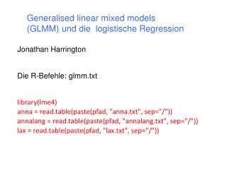
Logistische Regression und psychometrische Kurven Jonathan Harrington library(lme4) library(lattice) source(file.path(pfadu, "sigmoid.txt"))
Die Sigmoid-Funktion In der logistischen Regression wird eine sogenannte Sigmoid-Funktion an Proportionen angepasst. x ist die unabhängige Variable, m und k sind die Neigung und Intercept, p ist die eingeschätze Proportion. ^ In der logistischen Regression werden (m, k) berechnet, um den Abstand zwischen p (der tatsächlichen Proportion) und p zu minimieren. ^
DrittesBeispiel: numerischer UF ovokal = read.table(file.path(pfadu, "ovokal.txt")) Zwischen 1950 und 2005 wurde der Vokal in lost entweder mit hohem /o:/ oder tieferem /ɔ/ gesprochen. Ändert sich diese Proportion mit der Zeit? tab = with(ovokal, table(Jahr, Vokal)) prop = prop.table(tab, 1) barchart(prop, auto.key=T, horizontal=F) o = glm(Vokal ~ Jahr, family=binomial, data = ovokal)
Sigmoid überlagern (nur wenn der unabhängige Faktor wie hier numerisch ist) Proportionen berechnen k, m tab = with(ovokal, table(Jahr, Vokal)) glm() lmer() prop = prop.table(tab, 1) coef(o) Bevölkerung fixef(o) k, m berechnen, sigmoid überlagern Vpn-spezifisch k = coef(o)[1] coef(o)[[1]] m = coef(o)[2] sigmoid(prop, k, m) oder sigmoid(prop, k, m, rev=T)
Sigmoid Funktion und U-Punkte labr = read.table(file.path(pfadu, "labr.txt")) Ein Kontinuum zwischen /ʊ-ʏ/ wurde in 11 Schritten durch Herabstufung von F2 synthetisiert und eingebettet in einem /p_p/ Kontext. 20 Vpn. mussten entscheiden, ob ein Stimulus PUPP oder PÜPP war. Wo liegt der Umkipppunkt? Umkipppunkt: der F2-Wert, zu dem sich PUPP in PÜPP wandelt. tab.lab = with(labr, table(Stimulus, Urteil)) prop.lab = prop.table(tab, 1) barchart(prop.lab, auto.key=T, horizontal=F)
Sigmoid anpassen 1. Modell berechnen Berechnung von (k, m) pro Vpn o.lab = lmer(Urteil ~ Stimulus + (1+Stimulus|Vpn), family=binomial, data = labr) 2. k und m der Bevölkerung k.lab = fixef(o.lab)[1] m.lab = fixef(o.lab)[2] sigmoid(prop.lab, k.lab, m.lab) 3. U-Punkt = -k/m überlagern u.lab = -k.lab/m.lab abline(v=u.lab, lty=2) abline(h=.5, lty=2) 4. Vpn-spezifische k und m coef.lab = coef(o.lab)[[1]] 5. Vpn-spezifische U-Punkte (ein U-Punkt pro Vpn) um.lab = -coef.lab[,1]/coef.lab[,2]
Sigmoid anpassen Vpn-spezifische k und m coef.lab = coef(o.lab)[[1]] Vpn-spezifisch U-Punkte (ein Wert pro Vpn) um.lab = -coef.lab[,1]/coef.lab[,2] boxplot(um.lab)
Das gleiche für Alveolar durchführen alvr = read.table(file.path(pfadu, "labr.txt")) Dann die U-Punkte für Labial und Alveolar abbilden, wie unten: