Unsupervised Learning of Visual Object Categories: A Bayesian Approach

1. Unsupervised Learning of Visual Object Categories Michael Pfeiffer pfeiffer@igi.tugraz.at

2. References • M. Weber1, M. Welling1, P. Perona1 (2000) Unsupervised Learning of Models for Recognition • Li Fei-Fei1, R. Fergus2, P. Perona1 (2003) A Bayesian Approach to Unsupervised One-Shot Learning of Object Categories • (1 CalTech, 2 Oxford)

3. Question • Which image shows a face / car / …?

4. Visual Object Category Recognition • Easy for humans • Very difficult for machines • Large variability inside one category

5. To make it even more difficult … • Unsupervised • No help from human supervisor • No labelling • No segmentation • No alignment

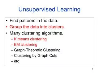
6. Topics • Constellation Model • Feature Selection • Model Learning (EM Algorithm) • Results, Comparison • One-shot Category Learning

7. Constellation Model (Burl, et.al.) • Object: Random constellation of Parts Shape / Geometry Part Appearance • Object class: Joint pdf on Shape and Appearance

8. Strength of Constellation Model • Can model Classes with strict geometric rules (e.g. faces) • Can also model Classes where appearance is the main criteria (e.g. spotted cats) Likely Unlikely

9. Recognition • Detect parts of the image • Form likely hypotheses • Calculate category likelihood Training • Decide on key parts of object • Select those parts in training images • Estimate joint pdf

10. Object Model • Object is a collection of parts • Parts in an image come from • Foreground (target object) • Background (clutter or false detections) • Information about parts: • Location • Part type

11. Probabilistic Model • Xo: „matrix“ of positions of parts from one image (observable) • xm: position of unobserved parts (hidden) • h: Hypothesis: which parts of Xo belong to the foreground (hidden) • n: Number of background candidates (dependent) • b: Which parts were detected (dependent) • p(Xo, xm, h) = p(Xo, xm, h, n, b)

12. Bayesian Decomposition p(Xo, xm, h, n, b) = p(Xo, xm|h, n)  p(h|n, b)  p(n)  p(b) • We assume independence between foreground and background (p(n) and p(b))

13. Models of PDF factors (1) • p(n) : Number of background part-detections • Mt: avg. Number of background (bg) detections of type t per image • Ideas: • Independence between bg parts • Bg parts can arise at every position with same probability Poisson Distribution

14. Models of PDF factors (2) • p(b) : 2F values for F features • b: Which parts have been detected • Explicit table of 2F joint probabilities • If F is large: F independent prob. • Drawback: no modelling of simultaneous occlusions

15. Models of PDF factors (3) • p(h | n, b) • How likely is a hypothesis h for given n and b? • n and b are dependent on h  Uniform distribution for all consistent hypotheses, 0 for inconsistent

16. Models of PDF factors (4) • p(Xo, xm | h, n) = pfg(z)  pbg(xbg) • z = (xo xm) : Coordinates of observed and missing foreground detections • xbg : Coordinates of all background detections • Assumption: foreground detections are independent of the background

17. Models of PDF factors (5) • pfg(z) : Foreground positions • Joint Gaussian with mean  and covariance matrix  • Translation invariant: Describe part positions relative to one reference part

18. Models of PDF factors (6) • pbg: positions of all background detections • Uniform distribution over the whole image of Area A

19. Recognition • Decide between object present (Class C1) and object absent (Class C2) • Choose class with highest a posteriori probabilityfrom observed Xo • h0: Null hypothesis: everything is bg noise • Localization is also possible!

20. Topics • Constellation Model • Feature Selection • Model Learning (EM Algorithm) • Results, Comparison • One-shot Category Learning

21. Part selection • Selecting parts that make up the model is closely related to finding parts for recognition • 1.: Finding Points of Interest • 2.: Vector quantization

22. Interest Operators • Förstner operator • Kadir-Brady operator • Well-known results from computer vision • Detect • Corner points • Intersection of lines • Centers of circular patterns • Returns ~150 parts per image • May come from background

23. Vector Quantization (1) • > 10.000 parts for 100 training images • k-means clustering of image patches • ~ 100 patterns • Pattern is average of all images in cluster

24. Vector Quantization (2) • Remove clusters with < 10 patterns: • pattern does not appear in significant number of training images • Remove patterns that are similar to others after 1-2 pixel shift • Calculate PCA of image patch • precalculated PCA basis

25. Result of Vector Quantization • Faces • Eyes, hairline, Mouth can be recognized • Cars • high-pass filtered • Corners and lines result from huge clusters

26. Topics • Constellation Model • Feature Selection • Model Learning (EM Algorithm) • Results, Comparison • One-shot Category Learning

27. Two steps of Model Learning • Model Configuration • How many parts make up the model? • Greedy search: Add one part and look if it improves the model • Estimate hidden Model Parameters • EM Algorithm

28. The EM Algorithm (1) • Expectation Maximization • Find a Maximum Likelihood Hypothesis for incomplete-data problems • Likelihood: • Find the most likely parameter vector  for (complete) observation X • What if X = (O, H) and only O is known?

29. The EM Algorithm (2) • p (O, H | ) = p(H | O, ) · p(O | ) • Likelihood L( | O, H) = p(O, H | ) is a function of random variable H • Define • Conditional expectation of log-likelihood depending on constants O and i-1

30. The EM Algorithm (3) • E – Step • Calculate Q( | i-1) using the current hypothesis i-1 and the observation O to model the distribution of H • M – Step • Find parameter vector i to maximize Q(i, i-1) • Repeat until convergence • Guaranteed to converge to local maximum

31. Hidden Parameters for This Model • : Mean of foreground part coordinates • : Covariance matrix of foreground detection coordinates • p(b): Occlusion statistics (Table) • M: Number of background detections • Observation: Xio coordinates of detections in images

32. Log-Likelihood Maximization • Use earlier decomposition of probabilistic model in 4 parts • Decompose Q into 4 parts • For every hidden parameter, only one part is dependent on it: maximize only this one! • Easy derivation of update rules (M – step) • Set derivation w.r.t. hidden parameter zero and calculate maximum point • Needed statistics calculated in E-step • Not shown here in detail

33. Topics • Constellation Model • Feature Selection • Model Learning (EM Algorithm) • Results, Comparison • One-shot Category Learning

34. Experiments (1) • Two test sets • Faces • Rear views of cars • 200 images showing the target • 200 background images • Random test and training set

35. Experiments (2) • Measure of success: • ROC : Receiver Operating Characteristics • X-Axis: False positives / Total Negatives • Y-Axis: True positives / Total Positives • Area under curve: • Larger area means: smaller classification error (good recall, good precision)

36. Experiments (3) • Number of parts: 2 – 5 • 100 learning runs for each configuration • Complexity: • EM converges in 100 iterations • 10s for 2 parts, 2 min for 5 parts • In total: Several hours • Detection: less than 1 second in Matlab

37. Results (1) • 93,5 % of all faces • 86,5 & of all cars correctly classified • Ideal number of parts visible • 4 for faces • 5 or more for cars

38. Results (2) • Appearance of parts in best performing models • Intuition not always correct • E.g. hairline more important than nose • For cars: often shadow below car is important, not tyres

39. Results (3) • Examples of correctly and incorrectly classified images

40. Related Work • R. Fergus, P. Perona, A. Zisserman (2003) Object Class Recognition by Unsupervised Scale-Invariant Learning • Straightforward extension of this paper • Even better results through scale invariance • More sophisticated feature detector (Kadir and Brady)

41. Characteristics of Classes

42. Topics • Constellation Model • Feature Selection • Model Learning (EM Algorithm) • Results, Comparison • One-shot Category Learning

43. One-shot learning Introducing the OCELOT

44. Jaguar Leopard Lynx Tiger OCELOT Serval Puma Can you spot the ocelot?

45. Biological Interpretation • Humans can recognize between 5000 and 30000 object categories • Humans are very quick at learning new object categories • We take advantage of prior knowledge about other object categories

46. Bayesian Framework • Prior information about objects modelled by prior pdf • Through a new observation learn a posterior pdf for object recognition • Priors can be learned from unrelated object categories

47. Basic idea • Learn a new object class from 1-5 new training images (unsupervised) • Builds upon same framework as before • Train prior on three categories with hundreds of training images • Learn new category from 1-5 images (leave-one-out)

48. Results: Face Class • General information alone is not enough • Algorithm performs slightly worse than other methods • Still good performance: 85-92% recognition • Similar results for other categories • Huge speed advantage over other methods • 3-5 sec per category

49. Summary • Using Bayesian learning framework, it is possible to learn new object categories with very few training examples • Prior information comes from previously learned categories • Suitable for real-time training

50. Future Work • Learn a larger number of categories • How does prior knowledge improve with number of known categories? • Use more advanced stochastic model