Download

1 / 22
220 likes | 424 Views
Adjusted R 2 , Residuals, and Review. Adjusted R 2 Residual Analysis Stata Regression Output revisited The Overall Model Analyzing Residuals Review for Exam 2. Exercise Review. Use the caschool.dta dataseet

E N D
Adjusted R2, Residuals, and Review • Adjusted R2 • Residual Analysis • Stata Regression Output revisited • The Overall Model • Analyzing Residuals • Review for Exam 2
Exercise Review • Use the caschool.dta dataseet • Run a model in Stata using Average Income (avginc) to predict Average Test Scores (testscr) • Examine the univariate distributions of both variables and the residuals • Walk through the entire interpretation • Build a Stata do-file as you go
Adjusted R2: An Alternative “Goodness of Fit” Measure • Recall that R2 is calculated as: • Hypothetically, as K approaches n, R2 approaches one (why?) – “degrees of freedom” • Adjusted R2 compensates for that tendency “explained sum of squares” “total sum of squares”
Calculating Adjusted R2 • The bigger the sample size (n), the smaller • the adjustment • The more complex the model (the bigger K • is), the larger the adjustment • The bigger R2 is, the smaller the • adjustment
Residual Analysis: Trouble Shooting • Conceptual use of residuals • e, or what the model can’t explain • Visual Diagnostics • Ideal: a “Sneeze plot” • Diagnostics using Residual Plots: • Checking for heteroscedasticity • Checking for non-linearity • Checking for outliers • Saving and Analyzing Residuals in Stata
ei ei=0 X Review: Assumptions Necessary for Estimating Linear Models 1. Errors have identical distributions Zero mean, same variance, across the range of X 2. Errors are independent of X and other ei 3. Errors are normally distributed
e Predicted Y The Ideal: Sneeze Splatter Problems: It is possible to “over-interpret” residual plots; it is also possible to miss patterns when there are large numbers of observations
Problem: Standard errors are not constant; hypothesis tests invalid Heteroscedasticity e Predicted Y
Problem: Biased estimated coefficients, inefficient model Non-Linearity e Predicted Y
Residuals for model with outliers deleted Possible Outliers Checking for Outliers Residuals for model using all data e Predicted Y Problem: Under-specified model; measurement error
Stata Regression Model: Regressing “testscr” onto “avginc”
Use the case ID number to find the relevant observation in the data set Examination of Residuals gsort e (or you can use “-e”) list observat testscr avginc yhat e in 1/5 . list observat testscr avginc yhat e in 1/5 +---------------------------------------------------+ observat testscr avginc yhat e --------------------------------------------------- 1. 393 683.4 13.567 650.8699 32.53016 2. 386 681.6 14.177 652.0157 29.5842 3. 419 672.2 9.952 644.0789 28.12111 4. 366 675.7 11.834 647.6143 28.08568 5. 371 676.95 12.934 649.6807 27.26921 +---------------------------------------------------+
Residuals v. Predicted Values Using an “ocular test,” non-linearity seems probable, but heteroscedasticity is not obvious here. But should we trust our eyeballs?
Formal Test for Non-linearity:Omitted Variables Tests whether adding 2nd, 3rd and 4th powers of X will improve the fit of the model: Y=b0+b1X+b2X2+b3X3+b4X4+e
Formal Tests for Heteroscedasticity Tests to see whether the squared standardized residuals are linearly related to the predicted value of Y: std(e2)=b0+b1(Predicted Y)
Case-wise Influence Analysis The Leverage versus Squared Residual Plot
What to Do? • Nonlinearity • Polynomial regression: try X and X2 • Variable transformation: logged variables • Use non-OLS regression (curve fitting) • Heteroscedasticity • Re-specify model • Omitted variables? • Use non-OLS regression (WLS) • Use robust standard errors • Influential and Deviant Cases • Evaluate the cases • Run with controls (multivariate model) • Omit cases (last option)
Next Week • Review regression diagnostics • Introduction to Matrix Algebra • Review for Exam