Part I – MULTIVARIATE ANALYSIS C4 ANOVA & MANOVA
170 likes | 488 Views
Part I – MULTIVARIATE ANALYSIS C4 ANOVA & MANOVA. © Angel A. Juan & Carles Serrat - UPC 2007/2008. 1.4.1: The F -Distribution (quick review). The F -distribution is basic to regression and analysis of variance.

Part I – MULTIVARIATE ANALYSIS C4 ANOVA & MANOVA
E N D
Presentation Transcript
Part I – MULTIVARIATE ANALYSIS C4 ANOVA & MANOVA © Angel A. Juan & Carles Serrat - UPC 2007/2008
1.4.1: The F-Distribution (quick review) • The F-distribution is basic to regression and analysis of variance. • The F-distribution has two parameters: the numerator, m, and denominator, n, degrees of freedom F(m,n) • Like the chi-square distribution, the F-distribution is skewed.
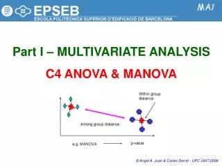
1.4.2: Overview of ANOVA & MANOVA • The main purpose of Analysis of Variance (ANOVA) is to test for significant differences among three or more means. This is accomplished by analyzing the variance, that is, by partitioning the total variance into the component that is due to true random error (within-group) and the components that are due to differences between means (among-group). If we are only comparing two means, then ANOVA will give the same results as the t test. • The variables that are measured (e.g., a test score) are called dependent or response variables. The variables that are manipulated or controlled (e.g., a teaching method or some other criterion used to divide observations into groups or levels that are compared) are called factors or independent variables. • Multivariate analysis of variance, MANOVA, is an extension of ANOVA methods to cover cases where there is more than one dependent variable. (# responses) (Levels in Factor/s) 1 response >=2 responses 2 levels 1 factor One-way ANOVA 2 factors Two-way ANOVA >=2 levels
1.4.3: Intro to ANOVA • A t-test can be used to compare two sample means. What if we want to compare more than two means? • Assume that we have k populations and that a random sample of size nj (j = 1, 2, …, k) has been selected from each of these populations. Analysis of Variance (ANOVA) can be used to test for the equality of the k population means: • Assumptions for ANOVA: • For each population, the response variable is normally distributed • The variance of the response variable, σ2, is the same for all the populations • The observations must be independent • Idea: If the means for the k populations are equal, we would expect the k sample means to be close together. ANOVA is a statistical procedure that can be used to determine whether the observed differences in the k sample means are large enough to reject H0 If H0 is rejected, we cannot conclude that all population means are different. Rejecting H0 means that at least two population means have different values. i.e.: if the variability among the sample means is “small”, it supports H0; if the variability among the sample means is “large”, it supports H1.
1.4.4: The Logic Behind ANOVA • A1= the assumptions for ANOVA are satisfied • A2 = the null hypothesis is true • On the one hand, under A1 & A2, each sample will have come from the same normal probability distribution with mean μ and variance σ2. Therefore, we can use the variability among the sample means* to develop the between-factors estimate of σ2 or MSF. • On the other hand, when a simple random sample is selected from each population, each of the sample variances provides an unbiased estimate of σ2. Hence, we can combine or pool the individual estimates of σ2into one overall estimate, called the pooled or within-factors estimateof σ2, MSE. • Under A1 & A2, the sampling distribution of MSF/MSE is an F( k – 1, nT – k ) distribution. Hence, we will reject H0 if the resulting value of MSF/MSE appears to be too large to have been selected at random from the corresponding F distribution. If H0 is true, MSF provides an unbiased estimate of σ2. However, if the means of the k populations are not equal, MSF is not unbiased. The MSE estimate is not affected by whether or not the population means are equal. It always provides an unbiased estimate of σ2. If H0 is true, the two estimates will be similar and MSF / MSE ≈ 1. If it is false, then MSF >> MSE.
1.4.5: One-way vs. Two-way ANOVA • One-way (one-factor) ANOVA compares several groups corresponding to a single categorical (independent) variable or factor, i.e.: one-way analysis of variance involves a single factor, which usually has three or more levels. Each level represents the treatment applied. • Two-way (two-factors) ANOVA performs an analysis of variance for testing the equality of populations means when classification of treatments is by two categorical (independent) variables or factors. Within each combination of the two factors or cell, you might have multiple observations called replicates. In two-way ANOVA, the data must be balanced, i.e.: all cells must have the same number of observations. In two-way ANOVA, possible interaction between the two factors (the effect that the two factors have on each other) must be considered. • Examples of one-way ANOVA applications: • In agriculture you might be interested in the effects of potassium (factor) on the growth of potatoes (response) • In medicine you might want to study the effects of medication (factor) on the duration of headaches (response) • In education you might want to study the effects of grade level (factor) on the time required to learn a skill (response) • A marketing experiment might consider the effects of advertising euros (factor) on sales (response) • Examples of two-way ANOVA applications: • In agriculture you might be interested in the effects of both potassium and nitrogen (factors) on the growth of potatoes (response) • In medicine you might want to study the effects of medication and dose (factors) on the duration of headaches (response) • In education you might want to study the effects of grade level and gender (factors) on the time required to learn a skill (response) • A marketing experiment might consider the effects of advertising euros and advertising medium (factors) on sales (response)
1.4.6: One-way ANOVA: Table (Minitab) In performing an ANOVA, you determine what part of the variance you should attribute to randomness and what part you can attribute to other factors. ANOVA does this by splitting the total sum of squares SST into two parts: a part due to random error SSE and a part attributed to differences between groups SSF. • File:SCORES.MTW • Stat > ANOVA > One-Way (Unstacked)... The CIs plot also shows that the 95%CI for the means of groups 1 and 3 are clearly disjoint. That suggest that groups 1 and 3 have different means. The Boxplots can help to visually detect differences among the populations being considered. • The ANOVA table shows the following calculations: • SS Factor, SS Error and SS Total • MS Factor and MS Error • Degrees of freedom (DF) associated with SSF and SSE • F statistic • p-value for the hypothesis test (reject H0 if p-value <= α)
1.4.7: One-way ANOVA: Checking assumpt. • File:SCORES.MTW When performing an ANOVA test, you assume that all the observations come from normally distributed populations. Obtaining a normal probability plotfor each sample group can be helpful in order to determine if it is reasonable to assume normality. In this case, it seems reasonable to assume that observations from Group 2 are normally distributed. For each sample group, a similar plots should be analyzed. To check for constant variance, use the graphical method of plotting the residuals versus the level or group. If the residuals (observed value – sample mean) have roughly the same range or vertical spread in each shift, then they satisfy the constant variance assumption. In this case, the constant variance assumption does not appear to be violated.
1.4.8: One-way ANOVA: Fisher’s LSD • Suppose that one-way ANOVA has provided statistical evidence to reject the null hypothesis of equal means. In this case, Fisher’s Least Significant Difference(LSD) is a multiple comparison procedure (i.e., it conducts statistical comparisons between pairs of population means) that can be used to determine where the differences occur: Fisher’s LSD procedure is based on the t test statistic for the two-population case. Fisher’s LSD procedure provides 95% CI estimates of the differences between each pair of means. In this example, the Fisher’s 95% CI for the difference between Group 1 and Group 3 does not contain the zero value. Therefore, both groups seem to have different means. The same can be said regarding the difference between Group 2 and Group 3.
1.4.9: One-way ANOVA: Bonferroni adjust. • Fisher’s LSD procedure is used to make several pairwise comparisons of the form H0: μi = μjvs. H1: μi ≠ μj. In each case, a significance level of α= 0.05 is used. Therefore, for each test, if the null hypothesis is true, the probability that we will make a Type I error is α= 0.05(particular Type I error rate), and the probability that we will not make a Type I error on each test is 1 – 0.05 = 0.95. • If we make C pairwise comparisons, the probability that we will not make a Type I error on any of the C tests is (0.95)(0.95)…(0.95) = 0.95C. Therefore, the probability of making at least one Type I error is 1 – 0.95C(overall Type I error rate). Note that the larger C the more close to 1 will be this error rate. • One alternative for controlling the overall Type I error rate, referred as the Bonferroni adjustment, involves using a smaller particular error rate for each test, i.e.: take particular = overall / C. Another alternative is to use Tukey’s procedure instead of Fisher’s LSD. Using Bonferroni adjustment: For instance, if we want to use Fisher’s LSD procedure test C= 3 pairwise comparisons with a a maximum overall error rate of 0.05, we set the particular error rate to be 0.05/3 = 0.017.
1.4.10: One-way ANOVA: Tukey’s procedure • Many practitioners are reluctant to use Bonferroni adjustment since performing individual tests with a very low particular Type I error rate increases the risk of making a Type II error. • Tukey’s procedure can be used as an alternative to Fisher’s LSD. Tukey’s procedure is more conservative than Fisher’s LSD procedure, since it makes it harder to declare any particular pair of means to be significantly different: Recall that, for a fixed sample size, any decrease in the probability of making a Type I error will result in an increase in the probability of making a Type II error, which corresponds to accepting the hypothesis that the two population means are equal when in fact they are not. Tukey’s procedure provides 95% CI estimates of the differences between each pair of means. In this example, the Tukey’s 95% CI for the difference between Group 1 and Group 3 does not contain the zero value. Therefore, both groups seem to have different means. Note that conclusions for the difference between Group 2 and Group 3 are different from those obtained using Fisher’s LSD.
1.4.11: Two-way ANOVA: Table (Minitab) A marketing department wants to determine which one of two magazines(Factor A, 2 levels) has the lowest ratio of full-page adds to the number of pages in the magazine (Response). It also wants to determine whether there has been a change in this ratio during the last three years (Factor B, 3 levels). • File:RATIO2.MTW • Stat > ANOVA > Two-Way... We want to test three sets of hypothesis: H0: There is no interaction between factors H1: There is an interaction between factors H0: There is no difference in the mean Response for different levels of Factor A H1: There is a difference in the mean Response for different values of Factor A H0: There is no difference in the mean Response for different levels of Factor B H1: There is a difference in the mean Response for different levels of Factor B In Minitab, use the Two-way ANOVA when you have exactly two factors. If you have three or more factors, use the Balanced ANOVA. Both the Two-way and Balanced ANOVA require that all combinations of factor levels (cells) have an equal number of observations, i.e., the data must be balanced. For a significance level of 0.05, the results indicate a nonsignificant interaction between year and magazine (p-value = 0.338). You conclude that the mean ad ratios are probably the same for the three years (p-value = 0.494). In addition, you conclude that the mean ad ratios for the two magazines are not the same (p-value = 0.012).