Manufacturing Process Analysis & Tool Design
S lip -line field theory and upper-bound analysis. Manufacturing Process Analysis & Tool Design. MM555. Dermot Brabazon and Marcin Lipowiecki. Introduction.

Manufacturing Process Analysis & Tool Design
E N D
Presentation Transcript
Slip-line field theory and upper-bound analysis Manufacturing Process Analysis & Tool Design MM555 Dermot Brabazon and Marcin Lipowiecki
Introduction Slip-line field theory is used to model plastic deformation in plane strain only for a solid that can be represented as a rigid-plastic body. Elasticity is not included and the loading has to be quasi-static. This method has been recently largely superseded by finite element method, but this theory can provide analytical solutions to a number of metal forming processes, and utilises plots showing the directions of maximum shear stress in a rigid-plastic body which is deforming plastically in plane strain. (3)
Assumptions Besides the usual assumptions that the metal is isotropic and homogeneous, the common approach to this subject usually involves the following: • the metal is rigid-perfectly plastic; this implies the neglect of elasticstrains and treats the flow stress as a constant, • deformation is by plane strain, • possible effects of temperature, strain rate, and time are not considered, • there is a constant shear stress at the interfacial boundary. Usually,either a frictionless condition or sticking friction is assumed. (3)
When the theory cannot be used The principal ways in which slip-line field theory fails to take account of the behaviour of real materials are: • it deals only with non-strain-hardening materials. Whilst strain-hardening can be allowed for incalculations concerned with loads in anapproximate way, the manner in which strain distribution is altered becauseof it is not always clear • there is no allowance for creep or strain-rate effects. The rate of deformation at each given point in space and in the deforming body is generallydifferent, and any effect this may have on the yield stress is ignored.
When the theory cannot be used (cont.) • allinertia forces are neglected and the problems treated as quasi-static, • in the forming operations which impose heavy deformations, most ofthe work done is dissipated as heat; the temperatures attained may affect thematerial properties of the body or certain physical characteristics in thesurroundings, e.g. lubrication Despite these shortcomings, the theory is extremely useful; it is very important, however, to remember its limitations and not to expect too high a degree of correlation between experimental and theoretical work.
Plane plastic strain Deformation which proceeds under conditions of plane strain is such thatthe flow or deformation is everywhere parallel to a given plane, saythe (x, y) plane in a system of three mutually orthogonal planes andthe flow is independent of z. Since elastic strains are neglected, the plastic strain increments (or strain-rates) may be written in terms of the displacements (or velocities) ux(x, y), vy(x, y), wz = 0, as below (1)
State of stress It follows from the Levy-Mises relation that τxzand τyzare zero and therefore that σzis a principal stress. Further, since έz= 0, then σ’z= 0 and hence σz= (σx + σy)/2 = p, say. Because the material is incompressible έx= - έyand each incremental distortion is thus a pure shear.The state of stress throughout the deforming material is represented by a constant yield shear stress k, and a hydrostatic stress -p which in general varies from point to point throughout the material. k is the yield shear stress in plane strain and the yield criterion for this condition is: where k = Y/2 for the Tesca criterion and k = Y/ for the Mises criterion. (2)
Mohr’s circle diagram for stress in plane plastic strain The state of stress at any point in the deforming material may be represented in the Mohr circle diagram A and B represent the stress states (- p, ±k) at a point on planes parallel to the slip-lines through that point.
Directions of maximum shear strain-rate For an isotropic material the directions of maximum shear strain-rate, represented by points A and B coincide with the directions of yield shear stress and that such directions are clearly directions of zero rate of extension or contraction. The loci of these directions of maximum shear stress and shear strain-rate form two orthogonal families of curves known as slip-lines. The stresses on a small curvilinear element bounded by slip-lines are shown below: (3)
Slip lines The slip-lines are labelled αandβas indicated. It is essential to distinguish between the two families of slip-lines, and the usual convention is that when the α-andβ- lines form a right handed co-ordinate system of axes, then the line of action of the algebraically greatest principal stress, σ1passes through the first and third quadrants. The anti-clockwise rotation, ø, of the α-line from the chosen x-direction is taken as positive.
Slip lines (cont.) In order to determine the load necessary for a particular plastic forming operation, first of all the slip-line field patterns must be obtained. This means that equations for the variation of palong both α- and β-linesmust be derived. Also, we must check that all velocity conditions along α- and β-lines are satisfied.
The Stress Equations The equations of equilibrium for plane strain are, with neglect of body forces: (3) The above stress components σx, σyand τxyexpressed in terms of p and k are: (4) p is the normal or hydrostatic pressure on the two planes of yield shear stress.
The Stress Equations (cont.) Differentiating and substituting from equation (4) in equation (3) we have: (5) If now the α- and β-lines are taken to coincide with 0xand 0y at 0, that we take ø= 0, equations (5) become: (6)
The Stress Equations (cont.) Thus, integrating (7) If the hydrostatic stress pcan be determined at any one point on a slip-line (for example at a boundary), it can be deduced everywhere else. Thus (8)
Relations governing hydrostatic stress along slip-lines (Hencky equations) The equations (8) are known as the Hencky equations and are equivalent to the equilibrium equations for a fully plastic mass stressed in plane strain. In general, the values of the constants C1 and C2 from equation (7) vary from one slip-line to another.
The velocity field (Geiringer equations) In figure shown belowuand v are the component velocities of a particle at a point O along a pair of α- and β-slip-lines the α-line being inclined at øto the Oxaxis of a pair of orthogonal cartesian axes through O.
The velocity field (Geiringer equations) cont. The components of the velocity of the particle uxand vyparallel to Ox and Oy, respectively, are then (9) Taking the x-direction at point 0 tangential to the α-line, i.e. ø = 0. (10)
The velocity field (Geiringer equations) cont. Since εx = ∂ux/∂x is zero along a slip-line similarly it can be shown that (11) (12) Physically, it may be imagined that small rods lying on the slip-line directions at a point do not undergo extension or contraction.
Simple slip-line field solution for extrusion through a perfectly smooth wedge-shaped die of angleα • Top half of extrusion only is shown symmetrical about centreline • (b) Stress systems at M. • (c) Hodograph to (a)
Simple slip-line field solution for extrusion through a perfectly smooth wedge-shaped die of angleαcont. • To calculate stress on die face. • (b) A square die; container wall and die face both perfectly smooth;r = 2/3. • (c) Stress system at M of for drawing.
Refrences • Johnson, W., Mellor, P. B., Engineering Plasticity, Ellis Hordwood Limited, 1983 • Hosford, W. F ., Metal forming: mechanics and metallurgy2nd ed . - Englewood Cliffs, N.J : Prentice Hall, 1993 • www.DoITPoMS.ac.uk, University of Cambridge