Fatigue Analysis in Engineering Simulations
Explore the concepts of high-cycle and low-cycle fatigue, stress-based approaches, constant amplitude loading, and stress-life curves in this comprehensive chapter on fatigue analysis in engineering simulations.

Fatigue Analysis in Engineering Simulations
E N D
Presentation Transcript
Appendix Twelve Fatigue Module
Chapter Overview • In this chapter, the use of the Fatigue Module add-on will be covered: • It is assumed that the user has already covered Chapter 4 Linear Static Structural Analysis prior to this chapter. • The following will be covered in this section: • Fatigue Overview • General Fatigue Procedure for Constant Amplitude, Proportional Loading Case • Variable Amplitude, Proportional Loading • Constant Amplitude, Non-Proportional Loading • The capabilities described in this section are applicable to ANSYS DesignSpace licenses and above with the Fatigue Module add-on license. March 29, 2005 Inventory #002215 A12-2
A. Fatigue Overview • A common cause of structural failure is fatigue, which is damage associated with repeated loading • Fatigue is generally divided into two categories: • High-cycle fatigue is when the number of cycles (repetition) of the load is high (e.g., 1e4 - 1e9). Because of this, the stresses are usually low compared with the material’s ultimate strength. Stress-based approaches are used for high-cycle fatigue. • Low-cycle fatigue occurs when the number of cycles is relatively low. Plastic deformation often accompanies low-cycle fatigue, which explains the short fatigue life. Generally speaking, strain-based approaches should be used for low-cycle fatigue evaluation. • In Simulation, the Fatigue Module add-on license utilizes a stress-basedapproach and is suitable for high-cycle fatigue. Some pertinent aspects of the stress-based approach will be discussed next. March 29, 2005 Inventory #002215 A12-3
B. Constant Amplitude Loading • As noted earlier, fatigue is due to repetitive loading: • When minimum and maximum stress levels are constant, this is referred to as constant amplitude loading. This is a much more simple case and will bediscussed first. • Otherwise, the loading is known as variable amplitude or non-constant amplitude and requires special treatment (discussedlater in Section C of this chapter). March 29, 2005 Inventory #002215 A12-4
C. Proportional Loading • The loading may be proportional or non-proportional: • Proportional loading means that the ratioof the principal stresses is constant, and the principal stress axes do not change over time. This essentially means that theresponse with an increase or reversal ofload can easily be calculated. • Conversely, non-proportional loading means that there is noimplied relationship betweenthe stress components. Typicalcases include the following: • Alternating between two differentload cases • An alternating load superimposedon a static load • Nonlinear boundary conditions March 29, 2005 Inventory #002215 A12-5
smax smin D. Stress Definitions • Consider the case of constant amplitude, proportional loading, with min and max stress values smin and smax: • The stress range Ds is defined as (smax- smin) • The mean stress sm is defined as (smax+ smin)/2 • The stress amplitude or alternating stress sais Ds/2 • The stress ratio R is smin/smax • Fully-reversed loading occurs when an equal and opposite load is applied. This is a case of sm = 0 and R = -1. • Zero-based loading occurs when a load is applied and removed. This is a case of sm = smax/2 and R = 0. March 29, 2005 Inventory #002215 A12-6
Linear Plot Logarithmic Plot The same data is shown here with both a linear and logarithmic plot. Because of the nature of the data, it is often easier to use a logarithmic plot to view the S-N curve. E. Stress-Life Curves • The relationship of loading to fatigue failure is captured with a stress-life or S-N curve: • If a component is subjected to a cyclic loading, the component may fail after a certain number of cycles because cracks or other damage will develop • If the same component is subjected to a higher load, the number of cycles to failure will be less • The stress-life curve or S-N curve shows the relationship of stress amplitude to cycles to failure March 29, 2005 Inventory #002215 A12-7
… Stress-Life Curves • The S-N curve is produced by performing fatigue testing on a specimen • Bending or axial tests reflect a uniaxial state of stress • There are many factors affecting the S-N curve, some of which are noted below: • Ductility of material, material processing • Geometry, including surface finish, residual stresses, and existence of stress-raisers • Loading environment, including mean stress, temperature, and chemical environment • For example, compressive mean stresses provide longer fatigue lives than zero mean stress. Conversely, tensile mean stresses result in shorter fatigue lives than zero mean stress. • The effect of mean stress raises or lowers the S-N curve for compressive and tensile mean stresses, respectively. March 29, 2005 Inventory #002215 A12-8
… Stress-Life Curves • Consequently, it is important to keep in mind the following: • A component usually experiences a multiaxial state of stress. If the fatigue data (S-N curve) is from a test reflecting a uniaxial state of stress, care must be taken in evaluating life • Simulation provides the user with a choice of how to relate results with S-N curves, including multiaxial stress correction • Stress Biaxiality results aid in evaluating results at given locations • Mean stress affects fatigue life and is reflected in the shifting of the S-N curve up or down (longer or shorter life at a given stress amplitude) • Simulation allows for input of multiple S-N curves (experimental data) for different mean stress or stress ratio values • Simulation also allows for different mean stress correction theories if multiple S-N curves (experimental data) are not available • Other factors mentioned earlier which affect fatigue life can be accounted for with a correction factor in Simulation March 29, 2005 Inventory #002215 A12-9
… Summary • The Fatigue Module add-on allows users to perform stress-based approach for high-cycle fatigue. • The following cases are handled by the Fatigue Module: • Constant amplitude, proportional loading (Section B) • Variable amplitude, proportional loading (Section C) • Constant amplitude, non-proportional loading (Section D) • The required input data is the material S-N curve: • The S-N curve is from a fatigue test and may be uniaxial in nature while the actual component being analyzed may be in a multiaxial state of stress • S-N curves are dependent on a number of factors, including the mean stress. S-N curves at different mean stress values can be input directly, or mean stress correction theories can be implemented. March 29, 2005 Inventory #002215 A12-10
F. Fatigue Procedure (Basic Case) • Performing a fatigue analysis is based on a linear static analysis, so not all steps will be covered in detail. • Fatigue analysis is automatically performed by Simulation after a linear static solution. • It does not matter whether the Fatigue Tool is added prior to or after a solution since fatigue calculations are performed independently of the stress analysis calculations. • Although fatigue is related to cyclic or repetitive loading, the results used are based on linear static, not harmonic analysis. Also, although nonlinearities may be present in the model, this must be handled with caution because a fatigue analysis assumes linear behavior. • In this section, the case of constant amplitude, proportional loading will be covered. Variable amplitude, proportional loading and constant amplitude, non-proportional loading will be covered later in Sections C and D, respectively. March 29, 2005 Inventory #002215 A12-11
… Fatigue Procedure • Steps in yellow italics are specific to a stress analysis with the inclusion of the Fatigue Tool: • Attach Geometry • Assign Material Properties, including S-N Curves • Define Contact Regions (if applicable) • Define Mesh Controls (optional) • Include Loads and Supports • Request Results, including the Fatigue Tool • Solve the Model • Review Results March 29, 2005 Inventory #002215 A12-12
… Geometry • Fatigue calculations support solid and surfacebodies only • Line bodies currently do not output stress results, so line bodies are ignored for fatigue calculations. • Line bodies can still be included in the model to provide stiffness to the structure, although fatigue calculations will not be performed on line bodies March 29, 2005 Inventory #002215 A12-13
Fatigue Material Properties • As with a linear static analysis, Young’s Modulus and Poisson’s Ratio are required material properties • If inertial loads are present, mass density is required • If thermal loads are present, thermal expansion coefficient and thermal conductivity are required • If a Stress Tool result is used, Stress Limits data is needed. This data is also used for fatigue for mean stress correction. • The Fatigue Module also requires S-N curve data in the material properties of the Engineering Data • The type of data is specified under “Life Data” (see next page) • The S-N curve data is input in “Alternating Stress vs. Cycles” • If S-N curve material data is available for different mean stresses or stress ratios, these multiple S-N curves may also be input March 29, 2005 Inventory #002215 A12-14
… Fatigue Material Properties • To add or modify fatigue material properties: March 29, 2005 Inventory #002215 A12-15
… Fatigue Material Properties • From the Engineering Data tab, the type of display and input of S-N curves can be specified • The Interpolation scheme can be “Linear,” “Semi-Log” (linear for stress, log for cycles) or “Log-Log” • Recall that S-N curves are dependent on mean stress. If S-N curves are available at different mean stresses, these multiple S-N curves can be input • Each S-N curve at different mean stresses can be input directly • Each S-N curve at different stress ratios (R) can input instead March 29, 2005 Inventory #002215 A12-16
… Fatigue Material Properties • Multiple S-N curves may be added by right clicking in the “Mean Value” field and adding new mean values. • Each new mean value will have its own alternating stress table March 29, 2005 Inventory #002215 A12-17
… Fatigue Material Properties • Material property information can be stored or retrieved from an XML file • To save material data to file, right-click on material branch and use “Export …” to save to an external XML file • Fatigue material properties will automatically be written to the XML file, along with all other material data • Some sample material property is available in the Simulation installation directory:C:\Program Files\Ansys Inc\v81\AISOL\CommonFiles\Language\en-us\EngineeringData\Materials • “Aluminum” and “Structural Steel” XML files contain sample fatigue data which can be used as a reference • Fatigue data varies by material and by test, so it is important that the user use fatigue data representative of his/her parts March 29, 2005 Inventory #002215 A12-18
Contact Regions • Contact regions may be included in fatigue analyses • Note that only linear contact – Bonded and No-Separation – should be included when dealing with fatigue for constant amplitude, proportional loading cases • Although nonlinear contact – Frictionless, Frictional, and Rough – can be included, this may no longer satisfy the proportional loading requirement. • For example, changing the direction or magnitude of loading may cause principal stress axes to change if separation can occur. • The user must use care and his/her own judgement if nonlinear contact is present • For nonlinear contact, the method for constant amplitude, non-proportional loading (Section D) may be used instead to evaluate fatigue life March 29, 2005 Inventory #002215 A12-19
Loads and Supports • Any load and support that results in proportional loading may be used. Some types of loads and supports do not result in proportional loading, however: • Bolt Load applies a distributed force on the compressive side of the cylindrical surface. In reverse, the loading should change to the reverse side of the cylinder (although it doesn’t). • Pretension Bolt Load applies a preload first then external loads, so it is a two-load step process. • Compression Only Support prevents movement in the ‘compressive’ normal direction only but does not restrain movement in the opposite direction. • These type of loads should not be used for fatigue calculations for constant amplitude, proportional loading March 29, 2005 Inventory #002215 A12-20
Request Results • Any type of result for stress analysis may be requested: • Stresses, strains, and deformation • Contact Tool results (if supported by license) • Stress Tool may also be requested • Additionally, to perform fatigue calculations, the Fatigue Tool needs to be inserted • Under the Solution branch, add “Tools > Fatigue Tool” from the Context toolbar • The Details view of the Fatigue Tool control solution options for fatigue calculations • A Fatigue Tool branch will appear, and fatigue contour or graph results may be added • These are various fatigue results, such as life and damage, which can be requested March 29, 2005 Inventory #002215 A12-21
… Request Results • After the fatigue calculation has been specified, fatigue results may be requested under the Fatigue Tool • Contour results include Life, Damage, Safety Factor, Biaxiality Indication, and Equivalent Alternating Stress • Graph results only involve Fatigue Sensitivity for constant amplitude analyses • Details of these results will be discussed shortly March 29, 2005 Inventory #002215 A12-22
From Section A, recall that Ratio=0 is the same as “Zero-Based” loading and Ratio=-1 is equivalent to “Fully Reversed” loading. The type of loading specifies the min and max amplitudes. The “History Data” loading type will be discussed in Section C, as it is variable amplitude loading. Loading Type • After the Fatigue Tool is inserted under the Solution branch, fatigue specifications may be input in Details view • The Type of loading may be specified between “Zero-Based,” “Fully Reversed,” and a given “Ratio” • A scale factor may also be input to scale all stress results March 29, 2005 Inventory #002215 A12-23
Mean Stress Effects • Recall that mean stresses affects the S-N curve. “Analysis Type” specifies the treatment of mean stresses: • “SN-None” ignores mean stress effects • “SN-Mean Stress Curves” uses multiple S-N curves, if defined • “SN-Goodman,” “SN-Soderberg,” and “SN-Gerber” are mean stress correction theories that can be used March 29, 2005 Inventory #002215 A12-24
One can consider this graph to be a ‘multiplier’ to the single defined S-N curve. The horizontal line is 1.0, but for tensile mean stresses, the defined S-N curve will shift down. 3 1 2 … Mean Stress Effects • It is advisable to use multiple S-N curves if the test data is available (SN-Mean Stress Curves) • However, if multiple S-N curves are not available, one can choose from three mean stress correction theories. The idea here is that the single S-N curve defined will be ‘shifted’ to account for mean stress effects: 1. For a given number of cycles to failure, as the mean stress increases, the stress amplitude should decrease 2. As the stress amplitude goes to zero, the mean stress should go towards the ultimate (or yield) strength 3. Although compressive mean stress usually provide benefit, it is conservative to assume that they do not (scaling=1=constant) March 29, 2005 Inventory #002215 A12-25
Mean Stress Effects • The Goodman theory is suitable for low-ductility metals. No correction is done for compressive mean stresses. • The Soderberg theory tends to be moreconservative than Goodman and is sometimes used for brittle materials. • The Gerber theory provides good fitfor ductile metals for tensile mean stresses, although it incorrectly predicts a harmful effect of compressive mean stresses, as shown on the left side of the graph • The default mean stress correction theory can be changed from “Tools menu > Options… > Simulation: Fatigue > Analysis Type” • If multiple S-N curves exist but the user wishes to use a mean stress correction theory, the S-N curve at sm=0 or R=-1 will be used. As noted earlier, this, however, is not recommended. March 29, 2005 Inventory #002215 A12-26
Strength Factor • Besides mean stress effects, there are other factors which may affect the S-N curve • These other factors can be lumped together into the Fatigue Strength [Reduction] Factor Kf, the value of which can be input in the Details view of the Fatigue Tool • This value should be less than 1 to account for differences between the actual part and the test specimen. • The calculated alternating stresses will be divided by this modification factor Kf, but the mean stresses will remain untouched. March 29, 2005 Inventory #002215 A12-27
Stress Component • It was noted in Section A that fatigue testing is usually performed on uniaxial states of stress • There must be some type of conversion of multiaxial state of stress to a single, scalar value in order to determine the cycles of failure for a stress amplitude (S-N curve) • The “Stress Component” item in the Details view of the Fatigue Tool allows users to specify how stress results are compared to the fatigue S-N curve • Any of the 6 components or max shear, max principal stress, or equivalent stress may also be used. A signed equivalent stress takes the sign of the largest absolute principal stress in order to account for compressive mean stresses. March 29, 2005 Inventory #002215 A12-28
Solving Fatigue Analyses • Fatigue calculations are automatically done after the stress analysis is performed. Fatigue calculations for constant amplitude cases usually should be very quick compared with the stress analysis calculations • If a stress analysis has already been performed, simply select the Solution or Fatigue Tool branch and click on the Solve icon to initiate fatigue calculations • There will be no output shown in the Worksheet tab of the Solution branch. • Fatigue calculations are done within Workbench. The ANSYS solver is not executed for the fatigue portion of an analysis. • The Fatigue Module does not use the ANSYS /POST1 fatigue commands (FSxxxx, FTxxxx) March 29, 2005 Inventory #002215 A12-29
Reviewing Fatigue Results • There are several types of Fatigue results available for constant amplitude, proportional loading cases: • Life • Contour results showing the number of cycles until failure due to fatigue • If the alternating stress is lower than the lowest alternating stress defined in the S-N curves, that life (cycles) will be used(in this example, max cycles to failure inS-N curve is 1e6, so that is max life shown) • Damage • Ratio of design life to available life • Design life is specified in Details view • Default value for design life can bespecified under “Tools menu > Options… > Simulation: Fatigue > Design Life” March 29, 2005 Inventory #002215 A12-30
… Reviewing Fatigue Results • Safety Factor • Contour result of factor of safety with respect to failure at a given design life • Design life value input in Details view • Maximum reported SF value is 15 • Biaxiality Indication • Stress biaxiality contour plot helps to determine the state of stress at a location • Biaxiality indication is the ratio of the smaller to larger principal stress (with principal stress nearest to 0 ignored). Hence, locations of uniaxial stress report 0, pure shear report -1, and biaxial reports 1. Recall that usually fatigue test data is reflective of a test specimen under uniaxial stress (although torsional tests would be in pure shear). The biaxiality indication helps to determine if a location of interest is in a stress state similar to testing conditions. In this example, the location of interest (center) has a value of -1, so it is predominantly in shear. March 29, 2005 Inventory #002215 A12-31
… Reviewing Fatigue Results • Equivalent Alternating Stress • Contour plot of equivalent alternating stress over the model. This is the stress used to query the S-N curve after accounting for loading type and mean stress effects, based on the selected type of stress • Fatigue Sensitivity: • A fatigue sensitivity chart displays how life, damage, or safety factor at the critical location varies with respect to load • Load variation limits can be input (including negative percentages) • Defaults for chart options available under “Tools menu > Options… Simulation: Fatigue > Sensitivity” March 29, 2005 Inventory #002215 A12-32
… Reviewing Fatigue Results • Any of the fatigue items may be scoped to selected parts and/or surfaces • Convergence may be used with contour results • Convergence and alerts not available with Fatigue Sensitivity plots since these plots provide sensitivity information with respect to loading (i.e., no scalar item can be referenced for convergence purposes). March 29, 2005 Inventory #002215 A12-33
… Reviewing Fatigue Results • The fatigue tool may also be used in conjunction with a Solution Combination branch • In the solution combination branch, multiple environments may be combined. Fatigue calculations will be based on the results of the linear combination of different environments. March 29, 2005 Inventory #002215 A12-34
Set up a stress analysis (linear, proportional loading) Define fatigue material properties, including S-N curve(s) Specify loading type and treatment of mean stress effects Solve and postprocess fatigue results … Summary • Summary of steps in fatigue analysis: March 29, 2005 Inventory #002215 A12-35 Model shown is from a sample Solid Edge part.
G. Fatigue: Variable Amplitude Case • In the previous section, constant amplitude, proportional loading was considered. This involved cyclic or repetitive loading where the maximum and minimum amplitudes remained constant. • In this section, variable amplitude, proportional loading cases will be covered. Although loading is still proportional, the stress amplitude and mean stress varies over time. March 29, 2005 Inventory #002215 A12-36
s time … Irregular Load History and Cycles • For an irregular load history, special treatment is required: • Cycle counting for irregular load histories is done with a method called rainflow cycle counting • Rainflow cycle counting is a techniquedeveloped to convert an irregular stresshistory (sample shown on right) to cycles used for fatigue calculations • Cycles of different mean stress (“mean”)and stress amplitude (“range”) are counted. Then, fatigue calculations are performed using this set of rainflow cycles. • Damage summation is performed via the Palmgren-Miner rule • The idea behind the Palmgren-Miner rule is that each cycle at a given mean stress and stress amplitude uses up a fraction of the available life. For cycles Ni at a given stress amplitude, with the cycles to failure Nfi, failure is expected when life is used up. • Both rainflow cycle counting and Palmgren-Miner damage summation are used for variable amplitude cases. March 29, 2005 Inventory #002215 A12-37 Detailed discussion of rainflow and Miner’s rule is beyond the scope of this course. Consult any fatigue textbook for details.
… Irregular Load History and Cycles • Hence, any arbitrary load history can be divided into a matrix (“bins”) of different cycles of various mean and range values • Shown on right is the rainflow matrix, indicating for each value of mean and range how many ‘cycles’ have been counted • Higher values indicate that more of those cycles are present in load history • After a fatigue analysis is performed, the amount of damage each “bin” (cycle) caused can be plotted • For each bin from the rainflow matrix, the amount of life used up is shown (percentage) • In this example, even though low range/mean cycles occur most frequently, the high range values cause the most damage. • Per Miner’s rule, if the damage sums to 1 (100%), failure will occur. March 29, 2005 Inventory #002215 A12-38
Set up a stress analysis (linear, proportional loading) Define fatigue material properties, including S-N curve(s) Specify loading history data and treatment of mean stress effects Specify number of bins for rainflow cycle counting Solve and review fatigue results, (e.g., damage matrix, damage contour, life contour, etc.) … Variable Amplitude Procedure • Summary of steps for variable amplitude case: March 29, 2005 Inventory #002215 A12-39
… Variable Amplitude Procedure • The procedure for setting up a fatigue analysis for the variable amplitude, proportional loading case is very similar to Section B, with two exceptions: • Specification of the loading type is different with variable amplitude • Reviewing fatigue results include verifying the rainflow and damage matrices March 29, 2005 Inventory #002215 A12-40
After specifying the external text file which contains points of loading, its plot will be displayed on the Worksheet tab. Note that once the text file is read in, the values are stored in Simulation. The data is not dynamic (i.e., changing values in the text file require re-reading them into Simulation). Sample history load data can be found in the installation directory:C:\Program Files\Ansys Inc\v81\AISOL\CommonFiles\Language\en-us\EngineeringData\Load Histories … Specifying Load Type • In the Details view of the Fatigue Tool branch, the load “Type” will be “History Data” • An external file can then be specified under “History Data Location”. This text file should contain points of the loading history for one set of “cycles” (or period) • Since the values in the history data text file represent multipliers on load, the “Scale Factor” can also be used to scale the loading accordingly. March 29, 2005 Inventory #002215 A12-41
… Specifying Infinite Life • In constant amplitude loading, if stresses are lower than the lowest limit defined on the S-N curve, recall that the last-defined cycle will be used. However, in variable amplitude loading, the load history will be divided into “bins” of various mean stresses and stress amplitudes. Since damage is cumulative, these small stresses may cause some considerable effects, even if the number of cycles is high. Hence, an “Infinite Life” value can also be input in the Details view of the Fatigue Tool to define what value of number of cycles will be used if the stress amplitude is lower than the lowest point on the S-N curve. • Recall that damage is defined as the ratio of cycles/(cycles to failure), so for small stresses with no number of cycles to failure on the S-N curve, the “Infinite Life” provides this value. • By setting a larger value for “Infinite Life,” the effect of the cycles with small stress amplitude (“Range”) will be less damaging since the damage ratio will be smaller. March 29, 2005 Inventory #002215 A12-42
Bin Size=10 Bin Size=32 Bin Size=64 … Specifying Bin Size • The “Bin Size” can also be specified in the Details view of the Fatigue Tool for the load history • The size of the rainflow matrix will be bin_size x bin_size. • The larger the bin size, the bigger the sorting matrix, so the mean and range can be more accurately accounted for. Otherwise, more cycles will be put together in a given bin (see graph on bottom). • However, the larger the bin size, the more memory and CPU cost will be required for the fatigue analysis. The bin size can range from 10 to 200. The default value is 32, and it can be changed in the Control Panel. March 29, 2005 Inventory #002215 A12-43
… Specifying Bin Size • As a side note, one can view that a single sawtooth or sine wave for the load history data will produce similar results to the constant amplitude case covered in Section B. • Note that such a load history will produce 1 count of the same mean stress and stress amplitude as the constant amplitude case. • The results may differ slightly than the constant amplitude case, depending on the bin size, since the way in which the range is evenly divided may not correspond to the exact values, so it is recommended to use the constant amplitude method if it applies. March 29, 2005 Inventory #002215 A12-44
… Quick Counting • Based on the comments on the previous slides, it is clear that the number of bins affects the accuracy since alternating and mean stresses are sorted into bins prior to calculating partial damage. This is called “Quick Counting” technique • This method is the default behavior because of efficiency • Quick Rainflow Counting may be turned off in the Details view. In this case, the data is not sorted into bins until after partial damages are found and thus the number of bins will not affect the results. • Although this method is accurate, it can be much more computationally expensive and memory-intensive. March 29, 2005 Inventory #002215 A12-45
… Solving Variable Amplitude Case • After specifying the requested results, the variable amplitude case can be solved in a similar manner as the constant amplitude case, in conjunction with or after a stress analysis has been performed. • Depending on the load history and bin size, the solution may take much longer than the constant amplitude case, although it should still be generally faster than a regular FEA solution (e.g., stress analysis solution). March 29, 2005 Inventory #002215 A12-46
… Reviewing Fatigue Results • Results similar to constant amplitude cases are available: • Instead of the number of cycles to failure, Life results report the number of loading ‘blocks’ until failure. For example, if the load history data represents a given ‘block’ of time – say, one week – and the minimum life reported is 50, then the life of the part is 50 ‘blocks’ or, in this case, 50 weeks. • Damage and Safety Factor are based on a Design Life input in the Details view, but these are also ‘blocks’ instead of cycles. • Biaxiality Indication is the same as the constant amplitude case and is available for variable amplitude loading. • Equivalent Alternating Stress is not available as output for the variable amplitude case. This is because a single value is not used to determine cycles to failure. Instead, multiple values are used, based on the loading history. • Fatigue Sensitivity is also available for the ‘blocks’ of life. March 29, 2005 Inventory #002215 A12-47
The two results shown here are scoped results from different parts of the same model, using the same load history. The left shows that most of the damage (though a small fraction overall) occurs at lower stress amplitudes while the right shows that most of the damage (a large percentage) occurs at the highest stress amplitudes. … Reviewing Fatigue Results • There are also results specific to variable amplitude cases: • The Rainflow Matrix, although not really a result per se, is available for output and was discussed earlier. It provides information on how the alternating and mean stresses have been divided into bins from the load history. • The Damage Matrix shows the damage at the critical location of the scoped entities. It reflects the amount of damage per bin which occurs. Note that the result is of the critical location of scoped part(s) or surface(s). March 29, 2005 Inventory #002215 A12-48
H. Fatigue: Non-Proportional Case • In Section B, the constant amplitude, proportional loading case was discussed. • In this section, constant amplitude, non-proportional loading will be covered. • The idea here is that instead of using a single loading environment, two loading environments will be used for fatigue calculations. • Instead of using a stress ratio, the stress values of the two loading environments will determine the min and max values. This is why this method is called non-proportional since one set of stress results is not scaled, but two are used instead. • Because two solutions are required, the use of the Solution Combination branch makes this possible. March 29, 2005 Inventory #002215 A12-49
… Non-Proportional Procedure • The procedure for the constant amplitude, non-proportional case is the same as the one for the constant amplitude, proportional loading situation with the following exceptions: 1. Set up two Environment branches with different loading conditions 2. Add a Solution Combination branch and specify the two Environments to use 3. Add the Fatigue Tool (and any other results) for the Solution Combination branch, and specify “Non-Proportional” for the loading Type. 4. Request fatigue results as normal and solve March 29, 2005 Inventory #002215 A12-50