Download
1 / 20
230 likes | 595 Views
MATERIALS SCIENCE & ENGINEERING. Part of. A Learner’s Guide. AN INTRODUCTORY E-BOOK. Anandh Subramaniam & Kantesh Balani Materials Science and Engineering (MSE) Indian Institute of Technology, Kanpur- 208016 Email: anandh@iitk.ac.in, URL: home.iitk.ac.in/~anandh.

E N D
MATERIALS SCIENCE & ENGINEERING Part of A Learner’s Guide AN INTRODUCTORY E-BOOK Anandh Subramaniam & Kantesh Balani Materials Science and Engineering (MSE) Indian Institute of Technology, Kanpur- 208016 Email:anandh@iitk.ac.in, URL:home.iitk.ac.in/~anandh http://home.iitk.ac.in/~anandh/E-book.htm FATIGUE Fatigue of Materials (Cambridge Solid State Science Series) S. Suresh Cambridge University Press, Cambridge (1998) Atlas of Fatigue Curves Ed.: Howard E. Boyer American Society of Metals, Metals Park, OH (1986)
Salient Features & Overview Points • It is observed that materials subjected to dynamic/repetitive/fluctuating load (stress) fail at a stress much lower than that required to cause fracture in a single application of a load. Damage of material due to varying load (of magnitude usually less than the yield stress) ultimately leading to failure is termed as fatigue of material (or fatigue failure). • It is estimated that fatigue accounts for ~90% of all service failures due to mechanical causes. Corrosion being the other major cause of failures. • The insidious part of the phenomenon of fatigue failure is that it occurs without any obvious warning. Usually, fatigue failures occur after considerable time of service. • The surface which has undergone fatigue fracture appears brittle without gross deformation at fracture (in the macroscale). • On a macroscopic scale the fracture surface is usually normal to the direction of the principal tensile stress. • Fatigue failure is usually initiated at a site of stress concentration (E.g. a notch in the specimen or an acicular inclusion). • The term fatigue is borrowed from human reaction of ‘tiredness’ due to repetitive work! • Fatigue testing is often conducted in bending or torsion mode (rather than tension/compression mode). Bending tests are easy to conduct. In pipes fatigue tests may be done by internal pressurization with a fluid. • If the stress have a origin in thermal cycling, then the fatigue is called thermal fatigue. • Note: Fatigue loading is sometimes used to get a sharp crack in a notched specimen→ Called fatigue pre-cracking.
Factors affecting fatigue failure • Three factors play an important role in fatigue failure: (i) value of tensile stress (maximum), (ii) magnitude of variation in stress, (iii) number of cycles. • Geometrical (specimen geometry) and microstructural aspects also play an important role in determining fatigue life (and failure). Stress concentrators from both these sources have a deleterious effect. Residual stress can also play a role. • A corrosive environment can have a deleterious interplay with fatigue. Sufficiently high maximum tensile stress Factors necessary to cause fatigue failure Large variation/fluctuation in stress Sufficiently large number of stress cycles
Funda Check If the value of the maximum stress experienced by the material is less than the yield stress, should not the material be in a purely elastic state? (Why does failure occur in fatigue loading?). • Let us consider a uniaxial tensile loading. We have already noted* that the yield stress (y) is the macroscopic yield stress and microscopic yielding (by slip) is initiated at a much lower stress value. In uniaxial loading this slip usually does not lead to any appreciable effects or damage to the material/component. • In cyclic loading, on the other hand due to reversal of slip direction, intrusions can be caused on the surface, which are like small surface cracks (precursors to a full blown crack). • Once a crack forms from these intrusions (due to further cyclic loading), local stress amplification takes place. • In the presence of the crack the relevant material property to be considered is fracture toughness. *Click here to know: “Where does yielding start?”
Types of stress cycles and parameters characterizing them • The pattern of loading experienced by a component may be complicated involving many frequencies and may include vibration (Fig.1 below). (If the frequency of loading is very high, it is referred to as vibration). • The ‘essential’ effect of such a loading can be understood by simpler loading patterns like the sinusoidal wave (Fig.2 below). Tests involving such loading are easy to conduct and the results obtained is easy to interpret. Fig.1 I. Completely reversed cycle of stress • The simplest loading one can conceive is a sinusoidal wave pattern loading, where the stress/load oscillates about a mean zero load/stress. The stress amplitude (a) is marked in the figure.
r max Tensile stress → m min Cycles → 0 II. Purely tensile cycles • The stress/load oscillation may be sinusoidal, but the mean stress/load may be such that the stress state during the entire cycle is tensile. Needless to say, for a given stress amplitude this type of loading is more severe (as maximum stress max is min+ r). Various parameters are defined in the equations below.
Tensile → 0 Cycles → ← Stress → ← Compressive III. Random stress cycles • The stress/load oscillation may be sinusoidal, but the mean stress/load may be such that the stress state during the entire cycle is tensile. Needless to say, for a given stress amplitude this type of loading is more severe (as maximum stress max is min+ r).
S-N Curve • Engineering fatigue data is usually plotted as a S-N curve. Here S is the stress and N the number of cycles to failure (usually fracture). The x-axis is plotted as log(N). • The stress plotted could be one of the following: a, max, min. Each plot is for a constant m, R or A. • It should be noted that the stress values plotted are nominal values and does not take into account local stress concentrations. • Most fatigue experiments are performed with m = 0 (e.g. rotating beam tests). • Typically the stress value chosen for the stress is low (< y) and hence S-N curves deal with fatigue failure at a large number of cycles (> 105 cycles). These are the high cycle fatigue tests. • It is to be noted that the nominal stress < y, but microscopic plasticity occurs, which leads to the accumulation of damage. • As obvious, if the magnitude of Stress increases the fatigue life decreases. • Low cycle fatigue (N < 104 or 105 cycles) tests are conducted in controlled cycles of elastic + plastic strain (strain control mode, instead of stress control).
S-N Curve • Broadly two kinds of S-N curves can be differentiated for two classes of materials. (1) those where a stress below a threshold value gives a ‘very long’ life (this stress value is called the Fatigue Limit / Endurance limit). Steel and Ti come under this category.(2) those where a decrease in stress increases the fatigue life of the component, but no distinct fatigue life is observed. Al, Mg, Cu come under this category. • From a application point of view having a sharp fatigue limit is useful (as keeping service stress below this will help with long life (i.e. large number of cycles) for the component). 400 Fatigue limit = Endurance limit Fatigue limit Stress below Fatigue limit give ‘infinite life’ 300 Mild steel No fatigue limit fatigue strength is specified for and arbitrary number of cycles (~ 108 cycles) 200 Bending stress (MPa) → Aluminium alloy 100 • Steel, Ti show fatigue limit • Al, Mg, Cu show no fatigue limit(Might show a limit, but prohibitive to conduct such long time tests!) Note that number of cycles is in log scale Number of cycles to failure (N)→ 0 105 106 108 107
S-N Curve: Basquin equation • S-N curve in the high cycle region can be described by the Basquin equation:where, a is the stress amplitude, p & C empirical constants. • The S-N curve is usually determined using 8-12 specimens. Starting with a stress of two-thirds of the static tensile strength of the material the stress is lowered till specimens do not fail in about 107 cycles. As expected, there is usually there is considerable scatter in the data.
Microstructural aspects of fatigue failure • One of the important ‘mysteries’ related to fatigue is: “how does fatigue failure occur if the stress value used is below the yield stress?”. • Fatigue failure occurs because of microscopic plasticity (which can occur below the yield stress) and damage accumulation with time (i.e. number of cycles of loading). • Four important stages of fatigue can be identified:1Crack initiation (in notched specimens this stage may be absent). This occurs mostly at surfaces or sometimes at internal interfaces. Crack initiation may take place within about 10% of the total life of the component. 2Stage-I crack growth (Slip-band* crack growth): growth of crack along planes of high shear stress. This can be viewed as essentially extension of the slip process which lead to crack formation (something like deepening of the crack formed). 3Stage-II crack growth: in this stage the crack grows along directions of maximum tensile stress. Hence, crack propagation is trans-granular.4Ductile failure: reduction in load bearing area (due to crack propagation) leads to ultimate failure. • The crack which forms after stage-1 can be removed by annealing (i.e. the damage is reversible at that stage). • In parallel with dislocation activity, fatigue loading can give rise to an increased concentration of vacancies (as compared to uniform loading). These vacancies can further play a role in processes like climb, over-aging of precipitates, etc. (depending on the material and context). Crack initiation Crack deepening Crack growth Failure * Region of ‘concentrated slip’.
Slip and fatigue crack initiation • When a specimen (Fig.1) is subjected to uniform loading (e.g. pure shear in Fig.2), dislocations moving on parallel slip planes leave the free surface of crystal/grain, giving rise to slip lines on the surface of the specimen (Fig.2). The surface steps in static loading are typically 100-100nm high. Slip is prevalent in all grains of the specimen uniformly. • In fatigue loading on the other hand some grains may show slip while others may not. Due to accumulation of slip, slip bands form (within about 5% of the total number of cycles to failure), which increase with number of cycles. The surface steps created in this case are fine (~1nm) and further due to oscillatory loading this can lead to extrusions (Fig.3) and intrusions (Fig.4). The intrusions can act like a notch, which is a stress concentrator and are a precursor to a full blown crack. Dynamic/fatigue loading Fig.1 Fig.3 Fine scale compared to static loading Static loading Fig.4 Fig.2
Fatigue crack propagation • Once a crack has formed its growth can be understood in two stages. (i)Stage-I. Growth along slip bands due to shear stress (which lead to the formation of the intrusions), which can be thought of as crack deepening. The extension of the crack is only a few grain diameters during this stage at the rate of few nm per cycle. (ii)Stage-II marks faster crack growth of microns per cycle and is dictated by the maximum normal stress present. Striations characteristic of fatigue crack propagation are seen in this stage (fatigue striations). Each striation is produced by one cycle of stress. Sometimes these striations are difficult to detect and hence if striations are not found it does not imply that fatigue crack propagation was absent. The standard mechanism used to explain this phenomenon is shown in figure below (the tensile part of the cycle). During the compressive portion of the cycle the crack faces tend to close and the blunted crack tends to re-sharpen. • The important portion of the fatigue failure is the Stage-II crack growth and hence understanding the same helps one predict the failure cycles/time and hence plan for fail safe design (the component can be replaced before the crack grows to a critical value leading to failure: the concept of preventive maintenance). Formation of double notch concentrating slip at 45 due to tensile loading tensile part of the cycle Crack tip extension and blunting Crack widening.
Fatigue crack propagation • As we have seen stage II crack growth occupies the predominant portion of the fatigue life of a sample/component. Empirically it is seen that the crack growth rate (da/dN) follows a double power law equation. • a→ the alternating stress • a → the crack length • A,B → constants • m → ranges from 2-4 • n → ranges from 1-2 • In terms of the total strain () this can be expressed as: • We have noted that once the crack nucleates (as has already happed in stage I), the relevant parameter characterizing the mechanical behaviour of the material is the stress intensity factor and not the stress (alone). So a logical plot should be between da/dN and the range of stress intensity factors(K)experienced by the specimen. • A range of K (i.e. K) has to be considered as we are in fatigue loading mode. • Use of K further gives a crucial link between fatigue and fracture mechanics. * Note: in compression K is not defined and hence Kcompression is taken to be zero. However, the compressive part of the loading is important from mechanistic and other points of view (including the time involved).
A plot of da/dN vs K can the divided into three regions. Region-1 → slow or negligible crack growth.Region-2 → stable crack growth with power law behaviour (linear behaviour between crack growth rate and log of stress intensity factor range (logK) (called Paris’ law)).Region-3 → unstable crack growth leading to failure (as Kmax exceeds the Kc of the material). • We have noted that the materials we are dealing with are ductile with appreciable crack tip blunting. • Often the size of the plastic zone are small and hence the concepts of Linear Elastic Fracture Mechanics (LEFM) and hence ‘K’ can be used as a characterizing parameter in fatigue. Approximately linear curve in region-2 • C → a constant in region-2 • K → (Kmax Kmin) • p → ~3 for steels, 3-4 Al alloys • It is important to note that S-N curves are usually determined with R = 1 (fully reversed stress cycles) and (da/dN)-K curves are determined with R = 0 (pulsating tension). Hence, comparison of data and curves should be done carefully.
Fractography • Often progress of fracture in due to fatigue loading is indicated in a fractograph by a series of rings (or ‘beach marks’).
Effect of Metallurgical Variables • Fatigue related properties are sensitive to: (i) specimen geometry (with special reference to stress raisers) (ii) microstructure (including residual stress and microstructural stress raisers)(iii) surface finish. • Smooth surface finish and compressive residual stress improve fatigue properties (i.e increase fatigue life). • In some cases correlation is found between properties determined from static tensile tests (like UTS) with that determined from fatigue testing (e.g. fatigue limit). However, there is no universality to the behaviour. • As we have observed localization of slip is a key feature of fatigue crack nucleation. This implies that if slip can be ‘spread out’ more uniformly (homogenization of slip) then fatigue life with improve. In low stacking fault energy (SFE) materials (like Ag), cross-slip is more difficult (as the spacing between partials is more) and hence obstacles cannot be overcome easily by cross-slip. The opposite is true for high SFE materials (like Al), where cross-slip can lead to a set of parallel slip planes operating extensively. High SFE material
Effect of Metallurgical Variables… • Further, in low SFE materials, the grain size plays an important role in determining the fatigue life. This role is important only under conditions of low stress (where number of cycles to failure is high and stage-I cracking is predominant). Under such circumstances the following relation is often observed: • In high SFE materials, dislocation cell structures form on deformation and these play a more important role in stage-I cracking as compared to grain size. • The presence of interstitial and substitutional alloying elements play an important role in determining the S-N curve (fatigue life). Interstitial solutes, which contribute to strain aging give rise to a fatigue limit in the S-N curve. Substitutional elements increase fatigue life without introducing a fatigue limit. Enhanced strain aging effect (due to increased solute content or aging time) gives tolerance to higher stress values, for a given fatigue life Interstitial solute elements (like C in steel) introduce fatigue limit due to strain aging For a given stress, more number of cycles to failure.