Download

1 / 47
470 likes | 644 Views
Statistical Tropical Cyclone Forecast Models. Mark DeMaria NOAA/NESDIS Center for Satellite Applications and Research. AMS Short Course Notes January 21, 2008. Outline. Introduction and Terminology Short history of NHC statistical TC models The SHIPS intensity model

E N D
Statistical Tropical Cyclone Forecast Models Mark DeMaria NOAA/NESDIS Center for Satellite Applications and Research AMS Short Course Notes January 21, 2008
Outline • Introduction and Terminology • Short history of NHC statistical TC models • The SHIPS intensity model • Application of linear regression • The TC rapid intensity index • Application of discriminant analysis • Advanced fitting techniques • Neural Networks and Genetic Algorithms • Class exercise
Why Use Statistical Models? • Standard NWP model limitations • Grid resolution • Predictability • Physical parameterizations • Treatment of terrain, local effects • Model biases • Statistical Models • Model Output Statistics (MOS) • Perfect Prog • Both based on linear regression • Classification • Linear discriminant analysis
Model Output Statistics (MOS) • y = a1x1 + a2x2 + … aNxN + b • y = Predicted quantity (dependent variable) • Surface temp, precipitation amount and type, visibility, etc • xi, i = 1, 2 … N • Quantities from model forecast related to y • Independent variables • Can also include past data and climate input, latitude, longitude, Julian Day, etc • ai, b = regression coefficients
MOS Regression Coefficients • Training sample • Several years of model forecasts • “Ground truth” observations • Independent validation data (if possible) • Can use cross validation if necessary • Least-squares fit E = ½(yn-On)2 n=1,2 … N, N=sample size Oi=observations, yn=linear model prediction Set E/b =0 and E/ai = 0 to get equations for regression coefficients
MOS Development • MOS Advantages • Direct relationship between predicted variable and model forecasts • Model biases corrected • Takes into account forecast degradation with time • MOS Disadvantages • Modelers almost never leave their models alone • Data and assimilation changes can also impact model performance and bias • Model forecast archive files are very large
“Perfect Prog” Approach • Use observations or analyses for regression model development • Use forecast fields for real-time prediction • Advantages • Don’t need an archive of forecasts • Prediction improves as model forecast improves • Disadvantages • Model forecast biases not corrected • Predictor forecast degradation with time not included
Tropical Cyclone Statistical Model Types • Statistical • Use only basic storm information at or before t=0 • lat, lon, max winds, Julian Day • Climatology and Persistence (CLIPER) models • Statistical-Synoptic • Add predictors from t=0 model fields (analyses) • Statistical-Dynamical • Add predictors from model forecasts • Near all statistical-dynamical TC models use perfect-prog approach
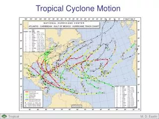
Long History of NHC Statistical Track Forecast Models • Riehl, Haggard, Sanborn (SS) 1959-1964 • Miller-Moore (SS) 1959-1964 • Travelers-59, -60 (SS) 1959-1964 • NHC-64, 67, 72 (SS) 1964-1988 • NHC-73, 83, 90, 98 (SD) 1973-2006 • HURRAN (S) 1970-1986 • CLIPER (S) 1971-present • 1970’s to early 1990’s was “Heyday” of SS and SD track models • Replaced by 3-D primitive equation models in 1990’s and 2000’s • S = statistical, SS=statistical synoptic, SD=statistical-dynamical • Underline= still run operationally at NHC
Shorter History of NHC Statistical Intensity Models • SHIFOR (S) 1988-present • SHIPS (SS) 1991-1995 • SHIPS (SD) 1996-present • SHIFOR = CLIPER-type intensity model • SHIPS = Statistical Hurricane Intensity Prediction Scheme • S = statistical, SS=statistical synoptic, SD=statistical-dynamical • Underline= still run operationally at NHC
Best Atlantic Intensity Models (48 hr error, 1988-2007) GFDL = NCEP version of GFDL coupled ocean-atmosphere hurricane model (Experimental in 1992, Operational in 1995) HWRF = follow-on to GFDL (Operational in 2007)
Current Statistical TC Forecast Techniques used by NHC • CLIPER and SHIFOR • Track and intensity forecast skill baseline models (regression) • SHIPS • SD intensity model (regression) • LGEM • hybrid dynamical, statistical model (regression for model growth rate) • Rapid Intensity Index • Discriminant analysis technique for classification • Annular Hurricane Index • Discriminant analysis technique for classification • Wind radii CLIPER • NESDIS version with idealized vortex (least squares for vortex fit) • NHC version (regression) • Rainfall CLIPER • Climatological rainfall rate along forecast track (least squares) • Tropical cyclone formation probability product • NESDIS product with discriminant analysis technique • Wind probability products • Monte Carlo technique to estimate probability of 34, 50 and 64 kt winds
Case Study: The Statistical Hurricane Intensity Prediction Scheme (SHIPS) • Original Motivation • Statistical Philosophy • Mathematical Formulation • Predictors • Model Performance
Statistical “Philosophy” • Use physical reasoning to select predictors • Especially for higher-order terms (quadratic, etc) • Require statistical significance at 1% level • Normalize variables so prediction coefficients are in units of standard deviations • Backwards stepwise procedure • Include at least one ENSO cycle in developmental sample • Perfect prog approach • Test on independent cases • Bill Gray, AT796 Tropical Meteorology • “Look at your data”
SHIPS Dependent Variable • Intensity is measured by maximum sustained 1-minute surface winds (V) • Predicted quantity is intensity change over give forecast interval • Separate regression equations for 0-6, 0-12, …, 0-120 hr forecasts • Sample restricted to storms over water • 1982-2006 sample • Kaplan and DeMaria (1995, 2001) inland decay model used over land
Physical Reasoning for Predictor Selection Hurricane Katrina August 2005
Physical Reasoning for Predictor Selection Hurricane Debby August 2000
2007 Atlantic SHIPS Dependent Variables (Predictors) • Climatology and Persistence type (1-4) • V at t=0 • V t=-12 to t=0 hours • Julian Day variable • Zonal component of storm motion • From GFS model analyses or forecasts (5-13) • 850-200 hPa vertical shear (0-500 km avg) • 200 hPa divergence (0-1000 km avg) • 850 hPa vorticity (0-1000 km avg) • 200 and 250 hPa temperature (200-800 km avg) • 700-500 avg hPa relative humidity (200-800 km avg) • Vertical instability parameter (200-800 km avg) • 850 hPa tangential wind change (0-600 km avg, 0 to fcst time) • Pressure where environmental winds best match storm motion
2007 Atlantic SHIPS Dependent Variables (Predictors) • From Reynold’s SST fields (14) • Maximum Potential Intensity at storm center minus initial intensity • From satellite data (15-16) • Std Deviation of IR brightness T (100-300 km) • Oceanic Heat Content at storm center (from satellite altimetry)
2007 Atlantic SHIPS Dependent Variables (Predictors) • Quadratic terms (17-21) • Square of SST potential • V(0)* V (t=-12) • V(0)*Shear • V(0)*GOES TB Std Dev • Shear*sine(latitude)
Statistical Calculations • Input for each forecast interval • Dependent variable yn = Vn n=1,2 …, N N = sample size • Independent variables xjn j=1,2 …, J J = no. of predictors (21) • Find sample mean and std deviation of yn and xjn • Calculate normalized dependent and independent variables _ Yn = (yn-y)/y , Similarly for xjn
Assume Linear Model • Yn = a1X1n + a2X1n + … aJXJn • Don’t need constant term with normalized input • Compare model predictions (Yn ) with observed intensity changes from NHC best track (On) • Find coefficients ai to minimize model error
Coefficient Calculation • Set E/aj = 0 for j=1,2 … J a = C-1b a = [a1, a2, …, aJ]T b = [b1, b2, …, bJ]T n=N bj = (1/N) (XjnOj) n=1 n=N Cij = (1/N) (XinXjn) = covariance matrix elements n=1 • Use standard statistical tests to calculate P-values for coefficients • Probability that the coefficient is significantly different than zero • Model R2 = Percent of variance of observations explained by the model
Predictor Magnitudes versus Forecast Interval for Shear and Persistence
SHIPS Output to Forecasters 1 * ATLANTIC SHIPS INTENSITY FORECAST * * GOES/OHC INPUT INCLUDED * * DEAN AL042007 08/17/07 00 UTC * TIME (HR) 0 6 12 18 24 36 48 60 72 84 96 108 120 V (KT) NO LAND 85 87 91 95 99 104 109 110 117 119 124 120 117 V (KT) LAND 85 87 91 95 99 104 109 110 117 119 124 79 84 V (KT) LGE mod 85 86 87 89 91 98 106 113 120 125 127 81 94 SHEAR (KTS) 14 10 9 6 6 5 3 6 6 7 9 9 7 SHEAR DIR 274 266 263 199 198 310 123 338 333 64 84 66 46 SST (C) 28.6 28.6 28.7 28.7 28.8 29.0 28.9 29.3 29.6 30.1 30.0 29.2 29.9 POT. INT. (KT) 149 149 150 150 151 154 153 160 165 173 172 157 170 ADJ. POT. INT. 158 155 156 155 155 158 157 164 167 173 168 152 164 200 MB T (C) -52.8 -52.9 -52.8 -52.1 -52.0 -52.4 -51.7 -51.9 -51.2 -51.1 -50.3 -50.2 -49.5 TH_E DEV (C) 11 11 11 12 11 8 10 10 11 8 11 9 10 700-500 MB RH 58 59 60 60 61 63 63 62 62 59 64 66 67 GFS VTEX (KT) 17 19 20 22 22 20 21 19 23 23 28 25 26 850 MB ENV VOR 14 14 14 29 28 59 94 73 79 65 84 80 87 200 MB DIV 54 52 48 61 17 31 49 64 76 60 77 81 48 LAND (KM) 504 415 427 436 328 277 182 100 164 352 150 -17 249 LAT (DEG N) 14.0 14.3 14.6 14.9 15.1 15.6 16.2 16.9 17.8 18.8 19.9 21.2 22.5 LONG(DEG W) 57.7 59.7 61.6 63.5 65.3 68.7 72.3 76.1 79.8 83.1 85.9 88.9 92.1 STM SPEED (KT) 21 19 19 18 17 17 18 19 17 15 15 16 16 HEAT CONTENT 70 70 72 66 72 55 104 95 134 130 134 29 62 FORECAST TRACK FROM OFCI INITIAL HEADING/SPEED (DEG/KT):275/ 22 CX,CY: -21/ 2 T-12 MAX WIND: 85 PRESSURE OF STEERING LEVEL (MB): 622 (MEAN=625) GOES IR BRIGHTNESS TEMP. STD DEV. 100-300 KM RAD: 14.1 (MEAN=20.0) % GOES IR PIXELS WITH T < -20 C 50-200 KM RAD: 92.0 (MEAN=69.0)
SHIPS Output to Forecasters 2 INDIVIDUAL CONTRIBUTIONS TO INTENSITY CHANGE 6 12 18 24 36 48 60 72 84 96 108 120 ------------------------------------------------------------------- SAMPLE MEAN CHANGE 1. 2. 3. 4. 6. 8. 9. 10. 11. 11. 12. 13. SST POTENTIAL 2. 5. 7. 9. 10. 9. 6. 3. 1. 0. -3. -6. VERTICAL SHEAR -1. -2. -2. -2. 0. 2. 5. 7. 9. 9. 10. 11. PERSISTENCE 0. -1. -1. -1. -1. -1. -1. -1. -1. -1. 0. 0. 200/250 MB TEMP. 0. 0. -1. -1. -2. -2. -3. -4. -5. -6. -7. -8. THETA_E EXCESS 0. 0. 0. 0. 0. 0. -1. -1. -1. -2. -2. -2. 700-500 MB RH 0. 0. 0. 0. 0. 0. 0. 0. 0. 0. -1. -1. GFS VORTEX TENDENCY 0. 1. 2. 2. 1. 2. 0. 3. 3. 7. 4. 4. 850 MB ENV VORTICITY 0. 0. 0. 0. 0. 1. 2. 2. 3. 3. 4. 4. 200 MB DIVERGENCE 0. 0. 1. 1. 1. 2. 3. 4. 4. 5. 6. 5. ZONAL STORM MOTION 0. 0. 1. 2. 3. 4. 5. 6. 7. 8. 9. 10. STEERING LEVEL PRES 0. 0. 0. 0. 0. 0. 0. 0. 0. 0. 0. 0. DAYS FROM CLIM. PEAK 0. 0. 0. 0. 0. 0. 0. 0. 0. -1. -1. -1. ------------------------------------------------------------------ SUB-TOTAL CHANGE 2. 5. 10. 14. 19. 23. 24. 29. 31. 35. 32. 29. SATELLITE ADJUSTMENTS ------------------------------------------------------------------ MEAN ADJUSTMENT 0. 0. 0. 0. -1. -1. -1. -1. -1. -1. -1. -2. GOES IR STD DEV 0. 0. 0. 0. 0. 0. 0. 0. 0. 0. 0. 0. GOES IR PIXEL COUNT 0. 1. 1. 1. 1. 0. 0. 0. 0. 0. 0. 0. OCEAN HEAT CONTENT 0. 0. 0. 0. 0. 1. 2. 3. 5. 6. 5. 4. -------------------------------------------------------------------- TOTAL ADJUSTMENT 0. 0. 0. 0. 0. 1. 1. 2. 3. 4. 3. 3. -------------------------------------------------------------------- TOTAL CHANGE (KT) 2. 6. 10. 14. 19. 24. 25. 32. 34. 39. 35. 32.
Forecast Evaluation • Evaluation of SHIPS, GFDL, NHC Official and SHIFOR forecasts for 5-year Atlantic sample (2003-2007) • Compare forecasts with NHC best track intensities • Mean Absolute Error • Bias • usually small for statistical models • Skill • Percentage reduction in forecast error relative to a baseline forecast • Climatology and Persistence model (SHIFOR) used for skill baseline
Rapid Intensity Index (RII) • Rapid Intensification (RI) defined by percentiles of intensity change PDF • 95th percentile of Atlantic sample = 30 kt • 90th percentile of Atlantic sample = 25 kt • Classification problem • How do you separate the two groups? • RI from non-RI • NHC’s operational Rapid Intensity Index • Based on linear discriminant analysis • Component of the SHIPS model
Linear Discriminant Analysis • Developmental data • Group classification • Is this an RI case or not? • Observations that help to distinguish between the two groups (discriminators xj) • SHIPS predictors for the 24 hour forecast • Discriminant function • Linear combination of discriminators d = a1x1 + a2x2 + … aJxJ
Discriminant Weights • Choose weights to maximize separation of mean inputs between the two groups • Maximize [aT(x1 - x2)]2/(aTCpoola) a = (a1, a2 … aJ)T x1= (x11, x21, … xJ1)T (group 1 means) x2= (x12, x22, … xJ2)T (group 2 means) Cpool = common covariance matrix for the two groups • Optimal weights: a = [Cpool]-1(x1 - x2)
Group Estimation • Average distance between the two groups m = ½(aTx1 + aTx2) • For given xo, calculate discriminate value do = aTxo If do≥ m, assign to group 1 If do < m, assign to group 2
Input for Operational RII • Previous 12 hr intensity change • 850-200 hPa vertical shear • 200 hPa divergence • SST potential – Initial intensity • 850-700 hPa relative humidity • GOES TB std deviation (100-300 km) • Percent GOES pixels colder than -30oC (50-200 km)
RII Output to Forecasters ** 2007 ATLANTIC RAPID INTENSITY INDEX AL042007 DEAN 08/17/07 00 UTC ** ( 25 KT OR MORE MAX WIND INCREASE IN NEXT 24 HR) 12 HR PERSISTENCE (KT): 0.0 Range:- 45.0 to 30.0 Scaled/Wgted Val: 0.6/ 0.9 850-200 MB SHEAR (KT) : 9.1 Range: 35.1 to 3.2 Scaled/Wgted Val: 0.8/ 0.6 D200 (10**7s-1) : 46.4 Range: -20.0 to 149.0 Scaled/Wgted Val: 0.4/ 0.4 POT = MPI-VMAX (KT) : 70.6 Range: 8.1 to 130.7 Scaled/Wgted Val: 0.5/ 1.0 850-700 MB REL HUM (%): 72.0 Range: 57.0 to 88.0 Scaled/Wgted Val: 0.5/ 0.1 % area w/pixels <-30 C: 87.0 Range: 17.0 to 100.0 Scaled/Wgted Val: 0.8/ 0.5 STD DEV OF IR BR TEMP : 14.1 Range: 37.5 to 5.3 Scaled/Wgted Val: 0.7/ 0.6 Scaled RI index= 4.4 Prob of RI= 30% is 2.4 times the sample mean(12%) Discrim RI index= 4.2 Prob of RI= 29% is 2.4 times the sample mean(12%)
Neural Network Transfer Function T(x) x T(x) = 1/(1 + e-x)
Example Start with training data consisting of observed intensity change (y) predicted by shear (w) and SST potential (x)
Example w h1 y x h2 Have neural network with inputs w,x, two hidden nodes and an output y h₁ = a₁T(x) + a₂T(w) h₂ = a₃T(x) + a₃T(w) y = b₁T(h₁) + b₂T(h₂)
Genetic Algorithms General search algorithms inspired by biology Solutions to problems are encoded Encoded solutions can be thought of as the DNA of the solution Initial population of randomly generated solutions is generated Each generation, solutions are evaluated using a “fitness” function Solutions with better fitness functions have a higher probability to breed
Genetic Algorithms Breeding performed by mixing solution encodings Encodings in the population can be randomly altered to mutate the population Optionally, the lowest performing members of the population can be culled and replaced Mutation and culling helps prevent getting stuck in local minima and maxima Process continued until a desired fitness has been reached or until a set number of generations have passed
Example Define error function: E = ∑(y - O) ² Encoding for GA is simply a list of neural network weights Randomly generate a population of neural network weights and run the GA using the error function as the fitness function Breeding performed by swapping random elements of two sets of network weights
Summary • NHC has long history of operational statistical tropical cyclone models • Statistical track models replaced by dynamical models • Intensity, structure, genesis models still used • Most developed from “perfect prog” approach • Most use multiple regression (e.g., SHIPS) or discriminant analysis (e.g., RII) • Statistical “by-products” also useful to forecasters • More sophisticated methods under development • Neural networks and genetic algorithms.
References • DeMaria, M., M. Mainelli, L.K. Shay, J.A. Knaff and J. Kaplan, 2005: Further Improvements in the Statistical Hurricane Intensity Prediction Scheme (SHIPS). Wea. Forecasting, 20, 531-543. • DeMaria, M., and J.M. Gross, 2003: Hurricane! Coping with Disaster, edited by Robert Simpson, Chapter 4: Evolution of Tropical Cyclone Forecast Models. American Geophysical Union, ISBN 0-87590-297-9, 360 p. • Kalnay, E., 2003: Atmospheric Modeling, Data Assimilation and Predictability. Cambridge University Press, ISBN 0-521-79629-6, 341 p. • Russell S and P. Norvig 2003:. Artificial Intelligence: A Modern Approach, Second Edition. Upper Saddle River, New Jersey: Pearson Education Inc, 1047 p. • Wilks, D.S., 2006: Statistical Methods in the Atmospheric Sciences, 2nd Edition. Academic Press, ISBN 13: 978-0-12-751966-1, 627 p.