Decision Tree Approach in Data Mining
Decision Tree Approach in Data Mining. What is data mining ? The process of extracting previous unknown and potentially useful information from large database Several data mining approaches nowadays Association Rules Decision Tree Neutral Network Algorithm. Decision Tree Induction.

Decision Tree Approach in Data Mining
E N D
Presentation Transcript
Decision Tree Approach in Data Mining • What is data mining ? • The process of extracting previous unknown and potentially useful information from large database • Several data mining approaches nowadays • Association Rules • Decision Tree • Neutral Network Algorithm
Decision Tree Induction A decision tree is a flow-chart-like tree structure, where each internal node denotes a test on an attribute, each branch represents an outcome of the test, and leaf nodes represent classes or class distribution.
Data Mining Approach - Decision Tree • a model that is both predictive and descriptive • can help identify which factors to consider and how each factor associated to a business decision • most commonly used for classification (predicting what group a case belongs to) • several decision tree induction algorithms, e.g. C4.5, CART, CAL5, ID3 etc.
Algorithm for building Decision Trees Decision trees are a popular structure for supervised learning. They are constructed using attributes best able to differentiate the concepts to be learned. A decision tree is built by initially selecting a subset of instances from a training set. This subset is then used by the algorithm to construct a decision tree. The remaining training set instances test the accuracy of the constructed tree.
If the decision tree classified the instances correctly, the procedure terminates. If an instance is incorrectly classified, the instance is added to the selected subset of training instances and a new tree is constructed. This process continues until a tree that correctly classify all nonselected instances is created or the decision tree is built from the entire training set.
Entropy (a) shows probability p range from 0 to 1 = log(1/p) (b) Shows probability of an event occurs = p log(1/p) (c) Shows probability of an expected value (occurs+not occurs) = p log(1/p) + (1-p) log (1/(1-p))
Training Process |-------- Data Preparation Stage --------|------- Tree Building Stage -------|--- Prediction Stage ---|
Basic algorithm for inducing a decision tree • Algorithm: Generate_decision_tree. Generate a decision tree from the given training data. • Input: The training samples, represented by discrete-valued attributes; the set of candidate attributes, attribute-list; • Output: A decision tree
Begin Partition (S) If (all records in S are of the same class or only 1 record found in S) then return; For each attribute Ai do evaluate splits on attribute Ai; Use best split found to partition S into S1 and S2 to grow a tree with two Partition (S1) and Partition (S2); Repeat partitioning for Partition (S1) and (S2) until it meets tree stop growing criteria; End;
Information Gain Difference between information needed for correct classification before and after the split. For example, before split, there are 4 possible outcomes represented in 2 bits in the information of A, B, …Outcome. After split on attribute A, the split results in two branches of the tree, and each tree branch represent two outcomes represented in 1 bit. Thus, choosing attribute A results in an information gain of one bit.
Classification Rule Generation • Generate Rules • rewrite the tree to a collection of rules, one for each tree leaf • e.g. Rule 1: IF ‘outlook = rain’ AND ‘windy = false’ THEN ‘play’ • Simplifying Rules • delete any irrelevant rule condition without affecting its accuracy • e.g. Rule R-: IF r1 AND r2 AND r3 THEN class1 • Condition: Error Rate (R-) without r1 < Error Rate (R) => delete this rule condition r1 • Resultant Rule: IF r2 AND r3 THEN class1 • Ranking Rules • order the rules according to the error rate
Decision Tree Rules Rules are more appealing than trees, variations of the basic tree to rule mapping must be presented. Most variations focus on simplifying and/or eliminating existing rules.
A rule created by following one path of the tree is: Case 1: If Age<=43 & Sex=Male & Credit Card Insurance=No Then Life Insurance Promotion = No The conditions for this rule cover 4 of 15 instances with 75% accuracy in which 3 out of 4 meet the successful rate. Case 2: If Sex=Male & Credit Card Insurance=No Then Life Insurance Promotion = No The conditions for this rule cover 5 of 6 instances with 83.3% accuracy Therefore, the simplified rule is more general and more accurate than the original rule.
C4.5 Tree Induction Algorithm • Involves two phases for decision tree construction • growing tree phase • pruning tree phase • Growing Tree Phase • a top-down approach which repeatedly build the tree, it is a specialization process • Pruning Tree Phase • a bottom-up approach which removes sub-trees by replacing them with leaves, it is a generalization process
Expected information before splitting Let S be a set consisting of s data samples. Suppose the class label attribute has m distinct values defining m distinct classes, Ci for i=1,..m. Let Si be the number of samples of S in class Ci. The expected information needed to classify a given sample Si is given by: m Info(S)= - Si log2Si i=1 S S Note that a log function to the base 2 is used since the information is encoded in bit
Expected information after splitting Let attribute A have v distinct values {a1, a2,…av}, and is used to split S into v subsets {S1,…Sv} where Sj contains those samples in S that have value aj of A. After splitting, then these subsets would correspond to the branches partitioned in S. v InfoA(S) = S1j+…+Smj Info(Sj) j=1 S Gain (A) = Info (S) – InfoA(S)
C4.5 Algorithm - Growing Tree Phase Let S = any set of training case Let |S| = number of classes in set S Let Freq (Ci, S) = number of cases in S that belong to class Ci Info(S) = average amount of information needed to identify the class in S Infox(S) = expected information to identify the class of a case in S after partitioning S with the test on attribute X Gain (X) = information gained by partitioning S according to the test on attribute X
C4.5 Algorithm - Growing Tree Phase Select Decisive Attribute for Tree Splitting ( Informational Gain Ratio ) m Info(S)= - Si log2Si i=1 S S v InfoA(S) = S1j+…+Smj Info(Sj) j=1 S Gain (X) = Info (S) – Infox (S)
C4.5 Algorithm - Growing Tree Phase Let S be the training set Info (S) = -9 log2 (9) - 5 log2 (5) = 0.42+0.52=0.94 14 14 14 14 Where log2(9/14)= log 2 log (9/14) InfoOutlook(S) = 5 (- 2 log2 (2) - 3 log2 (3) ) 14 5 5 5 5 + 4 (- 4 log2 (4) - 0 log2 (0) ) 14 4 4 4 4 + 5 (- 3 log2 (3) - 2 log2 (2) ) = 0.694 14 5 5 5 5 Gain (Outlook) = 0.94 - 0.694 = 0.246 Similarly,computed information Gain(Windy) =Info(S) - InfoWindy(S) = 0.94 - 0.892 = 0.048 Thus, decision tree splits on attribute Outlook with higher information gain. Root | Outlook | Sunny Overcast Rain
Decision Tree after grow tree phase Root | Outlook / | \ Sunny Overcast Rain / \ | / \ Wendy not Play Windy not wendy (100%) wendy / \ / \ Play not play Play not play (40%) (60%)
Continuous-valued data If input sample data consists of an attribute that is continuous-valued, rather than discrete-valued. For example, people’s Ages is continuous-valued. For such a scenario, we must determine the “best” split-point for the attribute. An example is to take an average of the continuous values.
C4.5 Algorithm - Pruning Tree Phase ( Error-Based Pruning Algorithm ) U25%(E,N) = Predicted Error Rate = the number of misclassified test cases * 100% the total number of test cases where E is no. of error cases in the class, N is no. of cases in the class
Case study of predicting student enrolment by decision tree • Enrolment Relational schema Attribute Data type ID Number Class Varchar Sex Varchar Fin_Support Varchar Emp_Code Varchar Job_Code Varchar Income Varchar Qualification Varchar Marital_Status Varchar
Student Enrolment Analysis • deduce influencing factors associated to student course enrolment • Three selected courses’ enrolment data is sampled: Computer Science, English Studies and Real Estate Management • with 100 training records and 274 testing records • prediction result • Generate Classification Rules • Decision tree - Classification Rule • Students Enrolment: 41 Computer Science, 46 English Studies and 13 Real Estate Management
Growing Tree Phase C4.5 tree induction algorithm gain ratio of all possible data attributes Note: Emp_code shows highest information gain, and thus is the top priority in decision tree.
Growing Tree Phase classification rules • Root • Emp_Code = Manufacturing (English Studies = 67%) • -Quali = Form 4 Form 5 (English studies = 100%) • -Quali = Form 6 or equi. (English studies = 100%) • -Quali = First degree (Computer science = 100%) • -Quali = Master degree (computer science = 100%) • Emp_Code = Social work (computer science = 100%) • Emp_Code = Tourism, Hotel (English studies = 67%) • Emp_Code = Trading (English studies = 75%) • Emp_Code = Property (Real estate = 100%) • Emp_Code = Construction (Real estate = 56%) • Emp_Code = Education (computer science = 73%) • Emp_Code = Engineering (Real estate = 60%) • Emp_Code = Fin/Accounting (computer science = 54%) • Emp_Code = Government (computer science = 50%) • Emp_Code = Info. Tech. (computer science = 50%) • Emp_code = Others (English studies= 82%)
Pruned Decision Tree • Given: Error rate of Pruned Sub-tree Emp_code = “Manufacturing” =3.34 • Non-Pruned Sub-tree • Condition Error Rate • Emp_Code=“Manufacturing” 0.75 • Quali = Form 4 and 5 1.11 • Quali = Form 6 0.75 • Quali = First Degree 0.75 • Total 3.36 • Note: Prune tree since Pruning Error rate 3.34 < no pruning error rate 3.36
Prune Tree Phase classification Rules • No. Rule Class • 1 IF Emp_Code = “Government” AND Income = “$250,000 - $299,999” Real Estate Mgt • 2 IF Emp_Code = “Tourism, Hotel” English Studies • 3 IF Emp_Code = “Education” Computer Science • 4 IF Emp_Code = “Others” English Studies • 5 IF Emp_Code = “Government” AND Income = “$150,000 - $199,999” English Studies • 6 IF Emp_Code = “Construction” AND Job_Code = “Professional, Technical” Real Estate Mgt • 7 IF Emp_Code = “Manufacturing” English Studies • 8 IF Emp_Code = “Trading” AND Sex = “Female” English Studies • 9 IF Emp_Code = “Construction” AND Job_Code = “Executive” Real Estate Mgt • 10 IF Emp_Code = “Engineering” AND Job_Code = “Sales” Computer Science • 11 IF Emp_Code = “Engineering” AND Job_Code = “Professional, Technical” Real Estate Mgt • 12 IF Emp_Code = “Government” AND Income = “$800,000 - $999,999” Real Estate Mgt • 13 IF Emp_Code = “Info. Technology” AND Sex = “Female” English Studies • 14 IF Emp_Code = “Info. Technology” AND Sex = “Male” Computer Science • 15 IF Emp_Code = “Social Work” Computer Science • 16 IF Emp_Code = “Fin/Accounting” Computer Science • IF Emp_Code = “Trading” AND Sex = “Male” Computer Science • IF Emp_Code = “Construction” AND Job_Code = “Clerical” English Studies
Simplify classification rules by deleting unnecessary conditions Pessimistic error rate is due to its disappearance is minimal If the condition disappears, then the error rate is 0.338.
Simplified Classification Rules • No. Rule Class • 1 IF Emp_Code = “Government” AND Income = “$250,000 - $299,999” Real Estate Mgt • 2 IF Emp_Code = “Tourism, Hotel” English Studies • 3 IF Emp_Code = “Education” Computer Science • 4 IF Emp_Code = “Others” English Studies • 5 IF Emp_Code = “Manufacturing” English Studies • 6 IF Emp_Code = “Trading” AND Sex = “Female” English Studies • 7 IF Emp_Code = “Construction” AND Job_Code = “Executive” Real Estate Mgt • 8 IF Job_Code = “Sales” Computer Science • 9 IF Emp_Code = “Engineering” AND Job_Code = “Professional, Technical” Real Estate Mgt • 10 IF Emp_Code = “Info. Technology” AND Sex = “Female” English Studies • 11 IF Emp_Code = “Info. Technology” AND Sex = “Male” Computer Science • 12 IF Emp_Code = “Social Work” Computer Science • 13 IF Emp_Code = “Fin/Accounting” Computer Science • IF Emp_Code = “Trading” AND Sex = “Male” Computer Science • IF Job_Code = “Clerical” English Studies • 16 IF Emp_Code = “Property” Real Estate • 17 IF Emp_Code = “Government” AND Income = “$200,000 - $249,999” English Studies • c
Ranking Rules After simplifying the classification rule set, the remaining step is to rank the rules according to their prediction reliability percentage defined as (1 – misclassify cases / total cases of the rule) * 100% For the rule If Employment = “Trading” and “Sex=‘female’” then class = “English Studies” Gives out 6 cases with 0 misclassify cases. Therefore, give out 100% reliability percentage and thus is ranked first rule in the rule set.
Success rate ranked classification rules No. Rule Class 1 IF Emp_Code = “Trading” AND Sex = “Female” English Studies 2 IF Emp_Code = “Construction” AND Job_Code = “Executive” Real Estate Mgt 3 IF Emp_Code = “Info. Technology” AND Sex = “Male” Computer Science 4 IF Emp_Code = “Social Work” Computer Science 5 IF Emp_Code = “Government” AND Income = “$250,000 - $299,999” Real Estate Mgt 6 IF Emp_Code = “Government” AND Income = “$200,000 - $249,999” English Studies 7 IF Emp_Code = “Trading” AND Sex = “Male” Computer Science 8 IF Emp_Code = “Property” Real Estate 9 IF Job_Code = “Sales” Computer Science 10 IF Emp_Code = “Others” English Studies 11 IF Emp_Code = “Info. Technology” AND Sex = “Female” English Studies 12 IF Emp_Code = “Engineering” AND Job_Code = “Professional, Technical” Real Estate Mgt 13 IF Emp_Code = “Education” Computer Science 14 IF Emp_Code = “Manufacturing” English Studies 15 IF Emp_Code = “Tourism, Hotel” English Studies 16 IF Job_Code = “Clerical” English Studies 17 IF Emp_Code = “Fin/Accounting” Computer Science
Data Prediction Stage ClassifierNo. of misclassify casesError rate(%) Pruned Decision Tree 81 30.7% Classification Rule set 90 32.8% Both prediction results are reasonable good. The prediction error rate obtained is 30%, which means nearly 70% of unseen test cases can have accurate prediction result.
Summary • “Employment Industry” is the most significant factor affecting an student enrolment • Decision Tree Classifier gives the best better prediction result • Windowing mechanism improves prediction accuracy
Reading Assignment “Data Mining: Concepts and Techniques” 2nd edition, by Han and Kamber, Morgan Kaufmann publishers, 2007, Chapter 6, pp. 291-309.
Lecture Review Question 11 • Explain the term “Information Gain” in Decision Tree. • What is the termination condition of Growing tree phase? • Given a decision tree, which option do you prefer to prune the resulting rule and why? • Converting the decision tree to rules and then prune the resulting rules. • Pruning the decision tree and then converting the pruned tree to rules.
CS5483 tutorial question 11 Apply C4.5 algorithm to construct a decision tree after first splitting for purchasing records from the following data after dividing the tuples into two groups according to “age”: one is less than 25, and another is greater than or equal to 25. Show all the steps and calculation for the construction. Location Customer Sex Age Purchase records Asia Male 15 Yes Asia Female 23 No America Female 20 No Europe Male 18 No Europe Female 10 No Asia Female 40 Yes Europe Male 33 Yes Asia Male 24 Yes America Male 25 Yes Asia Female 27 Yes America Female 15 Yes Europe Male 19 No Europe Female 33 No Asia Female 35 No Europe Male 14 Yes Asia Male 29 Yes America Male 30 No