Download
1 / 18
180 likes | 249 Views
Explore the importance of intermediate representations (IR) in compiler design. Learn about IR design decisions, categories, and conversion from parse trees to abstract syntax trees. Study auxiliary graph representations like Control-Flow Graphs (CFG) and Directed Acyclic Graphs (DAGs).

E N D
Lecture 12: Intermediate Representations Front-End Back-End Source code IR Object code Lexical Analysis Syntax Analysis Context- Sensitive Analysis • (from previous lectures) The Front-End analyses the source code. Today’s lecture: Intermediate Representations (IR): • The Intermediate Representation encodes all the knowledge that the compiler has derived about the source program. To follow: Back-End transforms the code, as represented by the IR, into target code. Recall: Middle-End, may transform the code represented by the IR into equivalent code that may perform more efficiently. Typically: HL IR HL IR LL IR LL IR Front-End HL optimis. Generate LLIR LL optimis. Back-End COMP30142 Lecture 12
About IRs, taxonomy, etc... • Why use an intermediate representation? • To facilitate retargeting. • To enable machine independent-code optimisations or more aggressive code generation strategies. • Design issues: • ease of generation; ease of manipulation; cost of manipulation; level of abstraction; size of typical procedure. • Decisions in the IR design have major effects on the speed and effectiveness of compiler. • A useful distinction: • Code representation: AST, 3-address code, stack code, SSA form. • Analysis representation (may have several at a time): CFG, ... • Categories of IRs by structure: • Graphical (structural): trees, DAGs; used in source to source translators; node and edge structures tend to be large. • Linear: pseudo-code for some abstract machine; large variation. • Hybrid: combination of the above. There is no universally good IR. The right choice depends on the goals of the compiler!
From Parse Trees to Abstract Syntax Trees Goal Expr • Why we don’t want to use the parse tree? • Quite a lot of unnecessary information... • How to convert it to an abstract syntax tree? • Traverse in postorder (postfix) • Use mkleaf and mknode where appropriate • Match action with grammar rule (Aho1 pp.288-289; Aho2, 5.3.1) Expr - Term Term Term * Factor Factor Factor y x 2 • 1. Goal Expr 5. Term Term * Factor • 2. Expr Expr + Term 6. | Term / Factor • 3. | Expr – Term 7. | Factor • 4. | Term 8. Factor number • 9. | id COMP30142 Lecture 12
Abstract Syntax Trees - An Abstract Syntax Tree (AST) is the procedure’s parse tree with the non-terminal symbols removed. Example: x – 2*y • The AST is a near source-level representation. • Source code can be easily generated: perform an inorder treewalk - first the left subtree, then the root, then the right subtree - printing each node as visited. • Issues: traversals and transformations are pointer-intensive; generally memory-intensive. • Example: Stmt_sequence stmt; Stmt_sequence | stmt • At least 3 AST versions for stmt; stmt; stmt x * 2 y stmt ; Seq. stmt stmt ; stmt stmt stmt stmt stmt stmt
AST real-world example (dHPF) (1[GLOBAL] ! 2 components in true-branch ((2[PROG_HEDR] ! 6 components in true-branch (3[VAR_DECL] 4[PROCESSORS_STMT] 5[DISTRIBUTE_DECL] (6[FORALL_STMT] (7[ASSIGN_STAT] 8[CONTROL_END] ) NULL ) 9[PROC_STAT] 10[CONTROL_END] ) NULL ) (11[PROC_HEDR] (12[VAR_DECL] 13[INHERIT_DECL] (14[LOGIF_NODE] ! both branchs are non empty (15[ASSIGN_NODE] 16[CONTROL_END] ) (17[ASSIGN_NODE] 18[CONTROL_END] ) ) 19[RETURN_STAT] 20[CONTROL_END] ) NULL ) NULL ) PROGRAM MAIN REAL A(100), X !HPF$ PROCESSORS P(4) !HPF$ DISTRIBUTE A(BLOCK) ONTO P FORALL (i=1:100) A(i) = X+1 CALL FOO(A) END SUBROUTINE FOO(X) REAL X(100) !HPF$ INHERIT X IF (X(1).EQ.0) THEN X = 1 ELSE X = X + 1 END IF RETURN END
Directed Acyclic Graphs (DAGs) + * A DAG is an AST with a unique node for each value Example: The DAG for x*2+x*2*y Powerful representation, encodes redundancy; but difficult to transform, not useful for showing control-flow. Construction: • Replace constructors used to build an AST with versions that remember each node constructed by using a table. • Traverse the code in another representation. Exercise: Construct the DAG for x=2*y+sin(2*x); z=x/2 * y x 2 COMP30142 Lecture 12
Auxiliary Graph Representations The following can be useful for analysis: • Control-Flow Graph(CFG): models the way that the code transfers control between blocks in the procedure. • Node: a single basic block (a maximal straight line of code) • Edge: transfer of control between basic blocks. • (Captures loops, if statements, case, goto). • Data Dependence Graph: encodes the flow of data. • Node: program statement • Edge: connects two nodes if one uses the result of the other • Useful in examining the legality of program transformations • Call Graph: shows dependences between procedures. • Useful for interprocedural analysis. COMP30142 Lecture 12
Examples / Exercises Draw the call graph of: void a() { … b() … c() … f() … } void b() { … d() … c() … } void c() { … e() … } void d() { … } void e() { … b() … } void f() { … d() …} Draw the control-flow graph of the following: Stmtlist1 if (x=y) stmtlist2 stmtlist1 else stmtlist3 stmtlist1 stmtlist4 stmtlist1 while (x<k) stmtlist2 stmtlist3 Draw the data dependence graph of: 1. sum=0 2. done=0 3. while !done do 4. read j 5. if (j>0) 6. sum=sum+j 7. if (sum>100) 8. done=1 9. else 10. sum=sum+1 11. endif 12.endif 13.endwhile 14.print sum what about:1. Do i=1,n 2. A(I)=a(3*I+10) COMP30142 Lecture 12
Three-address code A term used to describe many different representations: each statement is a single operator and at most three operands. Example: if (x>y) then z=x-2*y becomes: t1=load x t2=load y t3=t1>t2 if not(t3) goto L t4=2*t2 t5=t1-t4 z=store t5 L: … Advantages: compact form, makes intermediate values explicit, resembles many machines. Storage considerations (until recently compile-time space was an issue) x–2*yQuadruples(Indirect) Triples load r1,y load 1 y - load y loadi r2,2 loadi 2 2 - loadi 2 mult r3,r2,r1 mult 3 2 1 mult (1),(2) load r4,x load 4 x - load x sub r5,r4,r3 sub 5 4 3 sub (4),(3) Array addresses have to be converted to single memory access (see lecture 13), e.g., A[I] will require a ‘load I’ and then ‘t1=I*sizeof(I); load A+t1’
Other linear representations • Two address code is more compact: In general, it allows statements of the form x=x <op> y (single operator and at most two operands). load r1,y loadi r2,2 mult r2,r2,r1 load r3,x sub r3,r3,r2 • One address code (also called stack machine code) is more compact. Would be useful in environments where space is at a premium (has been used to construct bytecode interpreters for Java): push 2 push y multiply push x subtract COMP30142 Lecture 12
Some Examples • 1: Simple back-end compiler: • Code: CFG + 3-address code • Analysis info: value DAG (represents dataflow in basic block) • 2. Sun Compilers for SPARC: • Code: 2 different IRs • Analysis info: CFG+dependence graph+?? • High-level IRs: linked list of triples • Low-level IRs: SPARC assembly like operations • 3. IBM Compilers for Power, PowerPC: • Code: Low-level IR • Analysis info: CFG + value graph + dataflow graphs. • 4. dHPF compiler: • Code: AST • Analysis info: CFG+SSA+Value DAG+Call Graph (SSA stands for Static Single Assignment: same as 3-address code, but all variables have a distinct name every time they are defined; if they are defined in different control paths the statement x3=Ø(x1,x2) is used to combine the two definitions) Remark: • Many kinds of IR are used in practice. Choice depends... • But… representing code is half the story! • Symbol tables, constants table, storage map.
Symbol Tables: The key idea • Introduce a central repository of facts: • symbol table or sets of symbol tables • Associate with each production a snippet of code that would execute each time the parser reduces that production - action routines. Examples: • Code that checks if a variable is declared prior to use (on a production like Factorid) • Code that checks that each operator and its operands are type-compatible (on a production like TermTerm*Factor) • Allowing arbitrary code provides flexibility. • Evaluation fits nicely with LR(1) parsing. • Symbol tables are retained across compilation (carry on for debugging too) COMP30142 Lecture 12
What information is stored in the symbol table? What items to enter in the symbol table? • Variable names; defined constants; procedure and function names; literal constants and strings; source text labels; compiler-generated temporaries. What kind of information might the compiler need about each item: • textual name, data type, declaring procedure, storage information. Depending on the type of the object, the compiler may want to know list of fields (for structures), number of parameters and types (for functions), etc… In practice, many different tables may exist. Symbol table information is accessed frequently: hence, efficiency of access is critical! COMP30142 Lecture 12
Organising the symbol table • Linear List: • Simple approach, has no fixed size; but inefficient: a lookup may need to traverse the entire list: this takes O(n). • Binary tree: • An unbalanced tree would have similar behaviour as a linear list (this could arise if symbols are entered in sorted order). • A balanced tree (path length is roughly equal to all its leaves) would take O(log2n) probes per lookup (worst-case). Techniques exist for dynamically rebalancing trees. • Hash table: • Uses a hash function, h, to map names into integers; this is taken as a table index to store information. Potentially O(1), but needs inexpensive function, with good mapping properties, and a policy to handle cases when several names map to the same single index. COMP30142 Lecture 12
foo... qq... i... Bucket hashing (open hashing) • A hash table consisting of a fixed array of m pointers to table entries. • Table entries are organised as separate linked lists called buckets. • Use the hash function to obtain an integer from 0 to m-1. • As long as h distributes names fairly uniformly (and the number of names is within a small constant factor of the number of buckets), bucket hashing behaves reasonably well. COMP30142 Lecture 12
Linear Rehashing (open addressing) • Use a single large table to hold records. When a collision is encountered, use a simple technique (i.e., add a constant) to compute subsequent indices into the table until an empty slot is found or the table is full. If the constant is relatively prime to the table size, this, eventually, will check every slot in the table. • Disadvantages: too many collisions may degrade performance. Expanding the table may not be straightforward. a rehash b If h(a)=h(b) rehash (say, add 3). COMP30142 Lecture 12
Other issues • Choosing a good hash function is of paramount importance: • take the hash key in four-byte chunks, XOR the chunks together and take this number modulo 2048 (this is the symbol table size). What is the problem with this? • See the universal hashing function (Cormen, Leiserson, Rivest), Knuth’s multiplicative function… This is one of those cases we should pay attention to theory! • Lexical scoping: • Many languages introduce independent name scopes: • C, for example, may have global, static (file), local and block scopes. • Pascal: nested procedure declarations • C++, Java: class inheritance, nested classes • C++, Java, Modula: packages, namespaces, modules, etc… • Namespaces allow two different entities to have the same name within the same scope: E.g.: In Java, a class and a method can have the same name (Java has six namespaces: packages, types, fields, methods, local variables, labels) • The problems: • at point x, which declaration of variable y is current? • as parser goes in and out of scopes, how does it track y? allocate and initialise a symbol table for each level! COMP30142 Lecture 12
Conclusion • Many intermediate representations – there is no universally good one! A combination might be used! • Representing code is half the story - Hash tables are used to store program names. • Choice of an appropriate hash function is key to an efficient implementation. • In a large system it may be worth the effort to create a flexible symbol table. • Fully qualified names (i.e., file.procedure.scope.x) to deal with scopes is not a good idea (the extra work needed to build qualified names is not worth the effort). • Reading: Reading: Aho2, pp. 85-100, 357-370; Aho1 pp.287-293; 429-440; pp.463-472. Cooper, Chapter 5 (excellent discussion).