Download
1 / 26
260 likes | 414 Views
Optimal solutions to geodetic inverse problems in statistical and numerical aspects. Jianqing Cai Geodätisches Institut, Universität Stuttgart Session 6: Theoretische Geodäsie Geodätische Woche 2010 05.–07. Oktober 2010, Messe Köln. Geodätisches Institut – Universität Stuttgart.

E N D
Optimal solutions to geodetic inverse problems in statistical and numerical aspects JianqingCai Geodätisches Institut, Universität Stuttgart Session 6: Theoretische Geodäsie GeodätischeWoche 2010 05.–07. Oktober 2010, Messe Köln Geodätisches Institut – Universität Stuttgart
Main Topics 1.Geodetic data analysis 2.Fixed effects (G-M, Ridge, BLE, - weighted homBLE) 3.Regularizations 4.Mixed model (Combination method) 5.Conclusionsandfurtherstudies
1. Geodetic data analysis • Many diffenent developed independently in separate disciplines. • Some clear differences in terminology, philosophy and numerical implementation remain, • due to tradition and lack of interdisciplinary communication. • Statistical aspect: Estimation and inference • the data are modeled as stochastic • Standard statistical concepts, questions, and considerations such as bias, variance, mean-square error, identifiability, consistency, efficiency and various forms of optimality can be applied • ill-posed problems is related to the rank defect, etc. • Biased and unbiased estimations • Numerical aspect: Inverse and ill-posed problems • Applied mathematicians often are more interesting in existence,uniqueness, and construction, given an inifinite number of noise-free data, and stability given data contaminated by a deterministic disturbance. • Approach: Tykhonov-Phillips regularization and • numerical methods such as L-Curve (Hansen 1992) or the Cp-Plot (Mallows 1973). 2 2
2. The special linear Gauss-Markov model Special Gauss Markov model 1st moments 2nd moments
Best Linear Estimation (BLE) (R. Rao, 1972) For the GGM model (y, Aξ, Σy= σ2P-1), and let L′y be an estimator of ξ; TheMean Square Error(MSE) of L′yis: It is not a suitable criterion for minimizing, since it involves both the unknowns. Three possibilities: Choose an a priori valueofσ-1ξ, say γand substitute σ2V =σ2γγ′forξξ′; Ifξisconsideredas a random variable with a priori meandispersionE(ξξ′)= σ2V; beconsistoftwoparts, varianceandbias. The choiseofV in Frepresentsthe relative weight, whichisn.n.dandof rank greaterthanone. yields the BLE of ξ 4 4
α-weighted hybrid minimum variance- minimum bias estimation (homα-BLE) • The open problem to evaluate the regularization parameter • Ever since Tykhonov (1963) and Phillips (1962) introduced the hybrid minimum norm approximation solution (HAPS) of a linear improperly posed problem there has been left the open problem to evaluate the regularization factor λ; • In most applications of Tykhonov-Phillips type of regularization the weighting factor λ is determined by heurishicalmethods, such as by means of L-Curve (Hansen 1992) or the Cp-Plot (Mallows 1973). In literature also optimization techniques have been applied.
-weighted S-homBLE and A-optimal design of the regularization parameter λ According to Grafarend and Schaffrin (1993), updated by Cai (2004), a homogeneously linear α-weighted hybrid minimum variance-minimum bias estimation (α, S-homBLE) is based upon the weighted sum of two norms of type: namely
α,S-homBLE: bias vector: Theorem 1 α,S-homBLE, also called: ridge estimator Linear Gauss-Markov model: dispersion matrix: Mean Square Error matrix:
Figure 1. The relationship between the variance, the squared bias and the weighting factor α. The variacne term decrease as α increases, while the squared bias increase with α.
The geodetic inverse Problem: • Exact or strict Multicollinearity means • weak Multicollinearity means • Use the condition Number for diagnostics: • The weight factor α can be alternatively • determined by the A-optimal design of type Here we focus on the third case – the most meaningful one – "minimize the trace of the Mean Square Errormatrix
Theorem 2. A-optimal design of Let the average hybrid -weighted variance-bias norm of ( α, S-homBLE) with respect to the linear Gauss-Markov model be given by then follows byA-optimal designin the sense of
Tykhonov-Phillips regularization: Tykhonov-Phillips regularization is defined as the solution to the problem yields the normal equations system • Ridge regression (Hoerl and Kennard, 1970a, b). Ridge regression is defined as biased estimation for nonorthogonal problems with a Lagrangian function: or a equivalent statement: yields the normal equations system 11 11 11
Generalized Tykhonov-Phillips regularization: Tykhonov-Phillips regularization is defined as the solution to the problem What is the solution of generalized regularization ? Rewrite the objective function yields the right solution 12 12 12 12
Comparison of the determination of the regularization factor λ by A-optimal design and the ridge parameter k in ridge regression • Hoerl, Kennard and Baldwin (1975) have suggested that if A′A=Im, then a minimum meansquare error (MSE) is obtained if ridge parameter for multiple linear regression model: • This is just the special case of our general solution by A-optimal design of Corollary 3 under unit weight P and A’A=Im, yielding 13
3. Mixed model (Combination method) Theil & Goldberger (1961) and Theil (1963), Toutenburg(1982) and Rao & Toutenburg(1999)mixed estimator with additional information as stochastic linear restrictions: Linear Gauss-Markov model: The additional information: Stochastic linear restriction: Mixed model: The BLUUE estimator of the original G-M model: The BLUUE estimator of the mixed model: The dispersion matrix: • The use of stochastic restrictions leads to a gain in efficiency.
The light constraint solutions (Reigber, 1989) Light constraint with a priori information Light constraint model: BLUUE estimator of light constraint model: With the dispersion matrix: The objective function of light constraint solution: • The same as the objective function of the estimate with weighting parameters ! Difference between estimators of the mixed models andlight constraint models:
Combination and Regularization methods In order to solve the PGP by spectral domain stabilization, we use a priori information in terms of spherical harmonic coefficients. Augmenting the minimization of squared residuals r = Aξ – y by a parameter component ξ – ξ0 yields the normal equations system • The parameter denotes the regularization parameter. It balances the residual norm ||Aξ – y|| against the (reduced) parameter norm ||ξ – ξ0||. • Accounts for both regularization and combination, which is just the so-called generalized Tykhonov regularization in the case of α = 1! • When ξ0 = 0, i.e. the a priori information consisting of null pseudo-observables, This is the case of regularization. • Data combination in the spectral domain is achieved by incorporating non-trivial a priori information ξ0 0, yielding the mixed estimator with additional information as stochastic linear restrictions.
Biased and unbiased estimations in different aspects Numerical Analysis Statistical aspects Ridge regression, BLE and Light constraint solution Standard Tykhonov-Phillips regularization BLUUE estimator of Mixed model Biased Gen.Tykhonov-Phillips regularization Unbiased • This answer the relationship of these biased and unbiased solutions and estimators in numerical and statistical aspects. 17
4. Conclusions and further studies • Development of a rigorous approach to minimum MSE adjustment in • a Gauss-Markov Model, i.e. α -weighted S-homBLE; • Derivation of a new method of determining the optimal regularization parameter in uniform Tykhonov-Phillips regularization (-weighted S-homBLE) by A-optimal design in the general case; • It was, therefore, possible to translate the previous results for the α -weighted S-homBLE to the case of Tykhonov-Phillips regularization with remarkable success; • The optimal ridge parameter k in ridge regression as developed by Hoerl and Kennardin 1970s is just the special case of our general solution by A-optimal design. • Accounts for both regularization and combination, which is just the so-called generalized Tykhonov regularization! 18
In ordertodevelopand promote thegeneralityofinversionmethods, itisnecessarytostudythiskindproblemfromthefollowingaspects: • Statistical ordeterministicregularization; • Ridgeestimation; • Best linear estimation; • Mixed model; • Biasedorunbiasedestimations; • The criterion in derivationoftheinversionsolution: • MeansquareerroroftheestimtesMSE - Gauss´ssecondapproach • insteadofGauss´sfirstapproach • 7) Optimal solution.
Historical remark: Laplace (1810) distinguishesbetweenerrorsofobservaionsanderrorsofestimates, andpoints out that a theoryofestimationshouldbebased on a measureofderviationbetweentheestimateandthetruevalue. Gauss(1823) finally accepted Laplace’s criticism and indicates that if he were to rewrite the 1809 proof (LS), he would use the expected mean square error as optimality criterion. This means that estimation theory should be based on minimization of the error of estimation!