Download
1 / 31
310 likes | 341 Views
Learn to identify real roots of polynomial equations, analyze end behavior, describe graphs, and use maxima and minima of functions. Understand end behavior, turning points, local maxima, and local minima in polynomial functions.

E N D
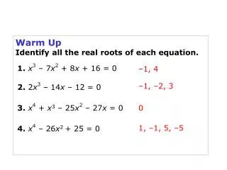
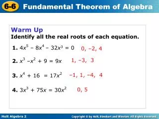
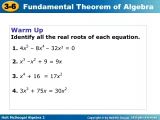
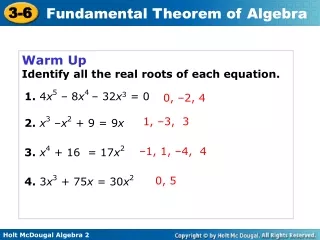
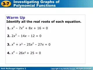
Warm Up Identify all the real roots of each equation. 1. x3 – 7x2 + 8x + 16 = 0 2. 2x3 – 14x – 12 = 0 3. x4 + x3– 25x2 – 27x = 0 4. x4 – 26x2 + 25 = 0
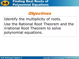
Objectives Use properties of end behavior to analyze, describe, and graph polynomial functions. Identify and use maxima and minima of polynomial functions to solve problems.
Vocabulary end behavior turning point local maximum local minimum
Polynomial functions are classified by their degree. The graphs of polynomial functions are classified by the degree of the polynomial. Each graph, based on the degree, has a distinctive shape and characteristics.
End behavior is a description of the values of the function as x approaches infinity (x +∞) or negative infinity (x –∞). The degree and leading coefficient of a polynomial function determine its end behavior. It is helpful when you are graphing a polynomial function to know about the end behavior of the function.
As x , P(x) , and as x , P(x) . As x , P(x) , and as x , P(x) . Example 1: Determining End Behavior of Polynomial Functions Identify the leading coefficient, degree, and end behavior. A. Q(x) = –x4+ 6x3 – x + 9 The leading coefficient is ____, which is _______. The degree is ___, which is ____. B. P(x) = 2x5+ 6x4 – x + 4 The leading coefficient is ____, which is _______. The degree is ___, which is ____.
As x , P(x) , and as x , P(x) . As x , P(x) , and as x , P(x) . Huddle Identify the leading coefficient, degree, and end behavior. a. P(x) = 2x5+ 3x2 – 4x –1 The leading coefficient is ___, which is _______. The degree is ___, which is ____. b. S(x) = –3x2+ x+ 1 The leading coefficient is ___, which is ________. The degree is ___, which is ____.
As x ___, P(x) , and as x , P(x) . Example 2A: Using Graphs to Analyze Polynomial Functions Identify whether the function graphed has an odd or even degree and a positive or negative leading coefficient. P(x) is of ___ degree with a _______ leading coefficient.
As x , P(x) , and as x , P(x) . Example 2B: Using Graphs to Analyze Polynomial Functions Identify whether the function graphed has an odd or even degree and a positive or negative leading coefficient. P(x) is of ____ degree with a ______ leading coefficient.
Huddle Identify whether the function graphed has an odd or even degree and a positive or negative leading coefficient.
Mastery Identify whether the function graphed has an odd or even degree and a positive or negative leading coefficient.
Now that you have studied factoring, solving polynomial equations, and end behavior, you can graph a polynomial function.
Example 3: Graphing Polynomial Functions Graph the function. f(x) = x3 + 4x2 + x – 6. Step 1Identify the possible rational roots by using the Rational Root Theorem. p = –6, and q = 1. Step 2 Test all possible rational zeros until a zero is identified. Test x = –1. Test x = 1.
5 5 2 2 f(0) = ___, so the y-intercept is __. Plot points between the zeros. Choose x = – , and x = –1 for simple calculations. f() = f(–1) = Example 3 Continued Step 3Write the equation in factored form. The zeros are ___, ___, ___. Step 4Plot other points as guidelines.
X , P(x) , and as x , P(x) . Example 3 Continued Step 5Identify end behavior. The degree is ____ and the leading coefficient is _______ so as Step 6Sketch the graph of f(x) = x3 + 4x2 + x – 6 by using all of the information about f(x).
Huddle Graph the function. f(x) = x3 – 2x2 – 5x + 6. Step 1Identify the possible rational roots by using the Rational Root Theorem. p = 6, and q = 1. Step 2 Test all possible rational zeros until a zero is identified. Test x = –1. Test x = 1.
Huddle Step 3Write the equation in factored form. The zeros are ___, ___, ____. Step 4Plot other points as guidelines. f(0) = ___, so the y-intercept is ___. Plot points between the zeros. Choose x = –1, and x = 2 for simple calculations. f(–1) = f(2) =
x , P(x) , and as x , P(x) . Huddle Step 5Identify end behavior. The degree is ____ and the leading coefficient is _______ so as Step 6Sketch the graph of f(x) = x3 – 2x2 – 5x + 6 by using all of the information about f(x).
Mastery Graph the function. f(x) = –2x2 – x + 6. Step 1Identify the possible rational roots by using the Rational Root Theorem. p = 6, and q = –2. Step 2 Test all possible rational zeros until a zero is identified.
Mastery Step 3The equation is in factored form. The zeros are ____, _____ . Step 4Plot other points as guidelines. f(0) = ____, so the y-intercept is ___. Plot points between the zeros. Choose x = –1, and x = 1 for simple calculations. f(–1) = f(1) =
x , P(x) , and as x , P(x) . Mastery Step 5Identify end behavior. The degree is _____ and the leading coefficient is _______ so as Step 6Sketch the graph of f(x) = –2x2 – x + 6 by using all of the information about f(x).
A turning point is where a graph changes from increasing to decreasing or from decreasing to increasing. A turning point corresponds to a local maximum or minimum.
A polynomial function of degree n has at most n – 1 turning points and at most n x-intercepts. If the function has n distinct roots, then it has exactly n – 1 turning points and exactly n x-intercepts. You can use a graphing calculator to graph and estimate maximum and minimum values.
25 –5 5 Step 2Find the maximum. Press to access the CALC menu. Choose 4:maximum.The local maximum is approximately ____________. –25 Example 4: Determine Maxima and Minima with a Calculator Graph f(x) = 2x3 – 18x + 1 on a calculator, and estimate the local maxima and minima. Step 1Graph. The graph appears to have one local maxima and one local minima.
Step 3Find the minimum. Press to access the CALC menu. Choose 3:minimum.The local minimum is approximately ___________. Example 4 Continued Graph f(x) = 2x3 – 18x + 1 on a calculator, and estimate the local maxima and minima.
5 –5 5 Step 2Find the maximum. Press to access the CALC menu. Choose 4:maximum.The local maximum is approximately _________. –5 Huddle Graph g(x) = x3 – 2x – 3 on a calculator, and estimate the local maxima and minima. Step 1Graph. The graph appears to have one local maxima and one local minima.
Step 3Find the minimum. Press to access the CALC menu. Choose 3:minimum.The local minimum is approximately __________. Huddle Graph g(x) = x3 – 2x – 3 on a calculator, and estimate the local maxima and minima.
10 –10 10 Step 3Find the minimum. Press to access the CALC menu. Choose 3:minimum.The local minimum is ______. –10 Mastery Graph h(x) = x4 + 4x2 – 6 on a calculator, and estimate the local maxima and minima. Step 1Graph. The graph appears to have one local maxima and one local minima. Step 2There appears to be _____ maximum.
Lesson Quiz: Part I 1. Identify whether the function graphed has an odd or even degree and a positive or negative leading coefficient.
Lesson Quiz: Part II Graph the function f(x) = x3 – 3x2 – x + 3. 2. 3. Estimate the local maxima and minima of f(x) = x3 – 15x – 2.